4.1: Exponential Functions

Learning Objectives

• Identify and evaluate exponential functions.
• Construct equations that model exponential growth.
• Use compound interest formulas and continuous growth and decay models.

India is the second most populous country in the world with a population of about \(1.25\) billion people in 2013. The population is growing at a rate of about \(.2\%\) each year. If this rate continues, the population of India will exceed China’s population by the year 2031. When populations grow rapidly, we often say that the growth is “exponential,” meaning that something is growing very rapidly. To a mathematician, however, the term exponential growth has a very specific meaning. In this section, we will take a look at exponential functions, which model this kind of rapid growth.

Identify Exponential Functions

When exploring linear growth, we observed a constant rate of change - a constant number by which the output increased for each unit increase in input (i.e. \(f(x+1) = f(x) \color{Cerulean}{ + c} \)). For example, in the linear equation \(f(x)=3x+4\), the difference in consecutive outputs, each time the input increases by \(1\), is always a constant, \(3\)  (notice \(3\) is the slope of the line). The scenario in the India population example is different - it exhibits exponential growth. In this situation, the ratio between consecutive outputs, each time \(1\) year goes by, is always a constant (i.e. \(f(x+1) = f(x) \color{Cerulean}{ \times c} \) ). In other words, each year, the number of people increases by a fixed percentage of the population. 

Exponential Functions

What exactly does it mean to grow exponentially? What does the word double have in common with percent increase? These words are often tossed around and appear frequently in the media.

• Percent change refers to a change based on a percent of the original amount. 
• Exponential growth refers to a percent increase of the original amount over time. The amount of increase is based on a constant multiplicative rate of change over equal increments of time.
• Exponential decay refers to a percent decrease of the original amount over time. The amount of decrease is based on a constant multiplicative rate of change over equal increments of time.

For us to gain a clear understanding of exponential growth, let us contrast exponential growth with linear growth. We will construct two functions. Both start with an input of \(0\). The first function is exponential. Every time the input is increased by \(1\) we will double the corresponding consecutive output. Thus the ratio between consecutive outputs will always be \(2\). The second function is linear. Every time the input is increased by \(1\) we will add \(2\) to the corresponding consecutive outputs. Thus the difference between consecutive output will always be \(2\). (Table \(\PageIndex{1}\)).

From Table \(\PageIndex{1}\) we can infer that for these two functions, exponential growth dwarfs linear growth.

• Exponential growth refers to the original value from the range increasing by the same percentage over equal increments found in the domain.
• Linear growth refers to the original value from the range increasing by the same amount over equal increments found in the domain.

Table \(\PageIndex{1. \text{ Exponential Growth vs. Linear Growth}}\)

\(x\)	0	1	2	3	4	5	6
\(f(x)=2^x\)	1	2	4	8	16	32	64
\(g(x)=2x\)	0	2	4	6	8	10	12

The next value, \(f(x+1)\) is 2 times more than the previous value \(f(x)\).
The next value, \(g(x+1)\) is an additional 2 more than the previous value \(g(x)\).

Clearly, the difference between “the same percentage” and “the same amount” is quite significant. For exponential growth, over equal increments, the constant multiplicative rate of change resulted in multiplying the output by \(2\) whenever the input increased by one. For linear growth, the constant additive rate of change over equal increments resulted in adding \(2\) to the output whenever the input was increased by one.

General form of the exponential function

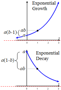
The general form of the exponential function is \(f(x)=ab^x\), where \(a\) is any nonzero number, \(b\) is a positive real number not equal to \(1\).

• The base, \(b\), is a constant called the growth factor, with \(b > 0\) and \(b \ne 1 \). 
  • If \(b>1\), the function grows at a rate proportional to its size.
  • If \(0<b<1\), the function decays at a rate proportional to its size.
• \(a\) is a constant called the initial value. It is called this because the value of \(f\) is \(a\) when \(x=0\)
  • the \(y\)-intercept is \((0, a)\).
  • the range is all positive real numbers \((0,\infty)\) if \(a>0\) and all negative real numbers \((-\infty, 0)\) if \(a<0\).
• An exponential function has a horizontal asymptote at \(y=0\)
• The independent variable \(x\) is in the exponent.
  • The exponent \(x\) can be any real number, so the domain of an exponential function is \((-\infty, \infty)\)

The base of an exponential function must be positive. The reason for this restriction ensures the outputs will be real numbers. Observe what happens if the base is not positive:

Let \(b=−9\) and \(x=\dfrac{1}{2}\). Then \(f(x)=f\left(\dfrac{1}{2}\right)={(−9)}^{\tfrac{1}{2}}=\sqrt{−9}\), which is not a real number.

The base of an exponential function cannot be \(1\). The reason for this restriction is because base \(1\) results in the constant function. Observe what happens if the base is \(1\):

Let \(b=1\). Then \(f(x)=1^x=1\) for any value of \(x\). The horizontal line \(y=1\) is not an exponential function!

Example \(\PageIndex{1}\): Identify Exponential Functions

Which of the following equations are not exponential functions?

\(f(x)=4^{3(x−2)}\)

\(g(x)=x^3\)

\(h(x)={\left(\dfrac{1}{3}\right)}^x\)

\(j(x)={(−2)}^x\)

Solution

By definition, an exponential function has a constant as a base and an independent variable as an exponent. Thus, \(g(x)=x^3\) does not represent an exponential function because the base is an independent variable. Functions like \(g(x)=x^3\) in which the variable is in the base and the exponent is a constant are called power functions.

Recall that the base \(b\) of an exponential function is always a positive constant, and \(b≠1\). Thus, \(j(x)={(−2)}^x\) does not represent an exponential function because the base, \(−2\), is less than \(0\).

 Try It \(\PageIndex{1}\)

Which of the following equations represent exponential functions?

\(f(x)=2x^2−3x+1\)

\(g(x)={0.875}^x\)

\(h(x)=1.75x+2\)

\(j(x)={1095.6}^{−2x}\)

Answer

\(g(x)={0.875}^x\) and \(j(x)={1095.6}^{−2x}\) represent exponential functions.

Evaluate Exponential Functions

To evaluate an exponential function with the form \(f(x)=b^x\), we simply substitute \(x\) with the given value, and calculate the resulting power. For example: Let \(f(x)=2^x\). What is \(f(3)\)?

\[\begin{align*} f(3)&= 2^3 &&\qquad \text{Substitute } x=3\\ &= 8 &&\qquad \text{Evaluate the power} \end{align*}\]

To evaluate an exponential function with a form other than the basic form, it is important to follow the order of operations. For example: Let \(f(x)=30{(2)}^x\). What is \(f(3)\)?

\[\begin{align*}  f(3)&= 30{(2)}^3 &&\qquad \text{Substitute } x=3\\ &= 30(8) &&\qquad \text{Simplify the power first}\\ &= 240 &&\qquad \text{Multiply} \end{align*}\]

Note that if the order of operations were not followed, the result would be incorrect: \(f(3)=30{(2)}^3≠{60}^3=216,000 \)

Example \(\PageIndex{2}\): Evaluate Exponential Functions

Let \(f(x)=5{(3)}^{x+1}\). Evaluate \(f(2)\) without using a calculator.

Solution: Follow the order of operations. Be sure to pay attention to the parentheses.

\[\begin{align*} f(2)&= 5{(3)}^{2+1} &&\qquad \text{Substitute } x=2\\ &= 5{(3)}^3 &&\qquad \text{Add the exponents}\\ &= 5(27) &&\qquad \text{Simplify the power}\\ &= 135 &&\qquad \text{Multiply} \end{align*}\]

Try It \(\PageIndex{2}\)

Let \(f(x)=8{(1.2)}^{x−5}\). Evaluate \(f(3)\) using a calculator. Round to four decimal places.

Answer \(5.5556\)

Exponential Growth Defined

Because the output of exponential functions increases very rapidly, the term “exponential growth” is often used in everyday language to describe anything that grows or increases rapidly. However, exponential growth can be defined more precisely in a mathematical sense. If the growth rate is proportional to the amount present, the function models exponential growth.

EXPONENTIAL GROWTH

A function that models exponential growth grows by a rate proportional to the amount present. For any real number \(a\) and \(x\), and any positive real number \(b\) such that \(b≠1\), an exponential growth function has the form

\[f(x)=ab^x \nonumber \]

where

• \(a\) is the initial or starting value of the function. In other words, \(f(0)=a\).
• \(b\) is the growth factor or growth multiplier per unit \(x\). In other words, \(f(x+1)=b \cdot f(x)\).
• \(b-1\) is the growth rate. It is the difference between outputs of consecutive values of \(x\). In other words, \(f(x+1) = f(x) + (b-1) \cdot f(x)\). If negative, there is exponential decay; if positive, there is exponential growth.

 

In more general terms, we have an exponential function, in which a constant base is raised to a variable exponent.

To differentiate between linear and exponential functions, let’s consider two companies, A and B. Company A has \(100\) stores and expands by opening \(50\) new stores a year, so its growth can be represented by the function \(A(x)=100+50x\). Company B has \(100\) stores and expands by increasing the number of stores by \(50\%\) each year, so its growth can be represented by the function \(B(x)=100{(1+0.5)}^x\).   A few years of growth for these companies are illustrated below. Table \(\PageIndex{3}\) Year, \(x\) Stores, Company A Stores, Company B \(0\) \(100+50(0)=100\) \(100{(1+0.5)}^0=100\) \(1\) \(100+50(1)=150\) \(100{(1+0.5)}^1=150\) \(2\) \(100+50(2)=200\) \(100{(1+0.5)}^2=225\) \(3\) \(100+50(3)=250\) \(100{(1+0.5)}^3=337.5\) \(x\) \(A(x)=100+50x\) \(B(x)=100{(1+0.5)}^x\) The graphs comparing the number of stores for each company over a five-year period are shown in Figure \(\PageIndex{2}\). We can see that, with exponential growth, the number of stores increases much more rapidly than with linear growth.   Notice that the domain for both functions is \([0,\infty)\),and the range for both functions is \([100,\infty)\). After year 1, Company B always has more stores than Company A.

Figure \(\PageIndex{2}\): The graph shows the numbers of stores Companies A and B opened over a five-year period.

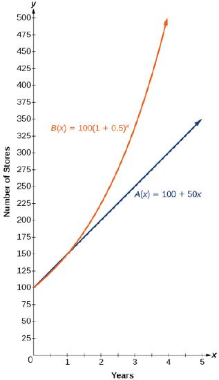
Now we will turn our attention to the function representing the number of stores for Company \(B\), \(B(x)=100{(1+0.5)}^x\). In this exponential function, \(100\) represents the initial number of stores, \(0.50\) represents the growth rate (the percent difference (as a decimal) between consecutive outputs), and \(1+0.5=1.5\) represents the growth factor (the growth multiplier per unit time). Generalizing further, we can write this function as \(B(x)=100{(1.5)}^x\), where \(100\) is the initial value, \(1.5\) is called the base, and \(x\) is called the exponent.

Example \(\PageIndex{3}\): Construct an Exponential Model Given the Growth Rate 

At the beginning of this section, we learned that the population of India was about \(1.25\) billion in the year 2013, with an annual growth rate of about \(1.2\%\). This situation is represented by the growth function \(P(t)=1.25{(1.012)}^t\), where \(t\) is the number of years since 2013. To the nearest thousandth, what will the population of India be in 2031?

Solution

To estimate the population in 2031, we evaluate the models for \(t=18\), because 2031 is \(18\) years after 2013. Rounding to the nearest thousandth,

\[P(18)=1.25{(1.012)}^{18}≈1.549 \nonumber\]

There will be about \(1.549\) billion people in India in the year 2031.

Try It \(\PageIndex{3}\)

The population of China was about \(1.39\) billion in the year 2013, with an annual growth rate of about \(0.6\%\). This situation is represented by the growth function \(P(t)=1.39{(1.006)}^t\), where \(t\) is the number of years since 2013. To the nearest thousandth, what will the population of China be for the year 2031? How does this compare to the population prediction we made for India in Example \(\PageIndex{3}\) ?

Answer

About \(1.548\) billion people; by the year 2031, India’s population will exceed China’s by about \(0.001\) billion, or \(1\) million people.

Construct Equations that Model Exponential Growth

In the previous examples, we were given an exponential function, which we then evaluated for a given input. Sometimes we are given information about an exponential function without knowing the function explicitly. We must use the information to first write the form of the function, then determine the constants \(a\) and \(b\), and evaluate the function.

How to: Given two data points, write an exponential model

1. If one of the data points has the form \((0,a)\), then \(a\) is the initial value. Using \(a\), substitute the second point into the equation \(f(x)=a{(b)}^x\), and solve for the growth factor, \(b\). The growth rate is \(b-1\).
2. If neither of the data points have the form \((0,a)\), substitute both points into two equations with the form \(f(x)=a{(b)}^x\). Solve the resulting system of two equations in two unknowns to find \(a\) and \(b\).
3. Using the \(a\) and \(b\) found in the steps above, write the exponential function in the form \(f(x)=a{(b)}^x\).

Example \(\PageIndex{4}\): Construct an Exponential Model when the Growth Rate is Not Given

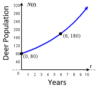
In 2006, \(80\) deer were introduced into a wildlife refuge. By 2012, the population had grown to \(180\) deer. The population was growing exponentially. Write an algebraic function \(N(t)\) representing the population \((N)\) of deer over time \(t\).

Solution

Choose the independent variable \(t\) be the number of years after 2006. This is done so that we can give ourselves an initial value for the function: when \(t=0\), \(a=80\). Thus, the information given in the problem can be written as input-output pairs: (0, 80) and (6, 180). We can now substitute the second point into the equation \(N(t)=80b^t\) to find \(b\):

\[\begin{align*} N(t)&= 80b^t\\ 180&= 80b^6 \qquad \text{Substitute using point } (6, 180)\\ \dfrac{9}{4}&= b^6 \qquad \text{Divide and write in lowest terms}\\ b&= {\left (\dfrac{9}{4} \right )}^{\tfrac{1}{6}} \qquad \text{Isolate b using properties of exponents}\\ b&\approx 1.1447 \qquad \text{Round to 4 decimal places} \end{align*}\]

To avoid rounding errors, do not round any intermediate calculations!. ONLY round the final answer. If the precision of the answer is not stated, give it to four digits.

The growth factor, \(b\), is \(1.1447\). The growth rate is \(1.1447-1 = .1447\) or \(14.47\%\)   The exponential model for the population of deer is \(N(t)=80{(1.1447)}^t\). (Note that this exponential function models short-term growth. As the inputs gets large, the predicted output will get so large that the model may not be useful.) We can graph our model to observe the population growth of deer in the refuge over time. Notice that the graph in Figure \(\PageIndex{3}\) passes through the initial points given in the problem, \((0, 80)\) and \((6, 180)\). We can also see that the domain for the function is \([0,\infty)\),and the range for the function is \([80,\infty)\).

Figure \(\PageIndex{3}\): Graph showing the population of deer over time, \(N(t)=80{(1.1447)}^t\), \(t\) years after 2006

Try It \(\PageIndex{4}\)

A wolf population is growing exponentially. In 2011, \(129\) wolves were counted. By 2013, the population had reached \(236\) wolves. What two points can be used to derive an exponential equation modeling this situation? Write the equation representing the population \(N\) of wolves over time \(t\).

Answer

\((0,129)\) and \((2,236)\); \(N(t)=129{(1.3526)}^t\)

Example \(\PageIndex{5}\): Construct an Exponential Model When the Initial Value is Not Known

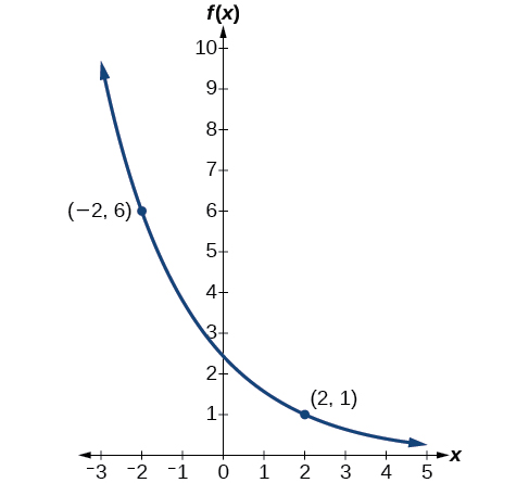
Find an exponential function that passes through the points \((−2,6)\) and \((2,1)\).

Solution

Because we don’t have the initial value, we substitute both points into an equation of the form \(f(x)=ab^x\), and then solve the system for \(a\) and \(b\).

• Substituting \((−2,6)\) gives \(6=ab^{−2}\)
• Substituting \((2,1)\) gives \(1=ab^2\)

Use the first equation to solve for \(a\) in terms of \(b\):

\[\begin{align*} 6&= ab^{-2}\\ \dfrac{6}{b^{-2}}&= a \qquad \text{Divide}\\ a&= 6b^2 \qquad \text{Use properties of exponents to rewrite the denominator} \end{align*}\]

Substitute \(a\) in the second equation, and solve for \(b\):

\[\begin{align*} 1&= ab^{2} = ({\color{red}{6b^2}}) b^2= 6 b^4 \qquad \text{Substitute a}\\ b&= \left (\dfrac{1}{6} \right )^{\tfrac{1}{4}} \qquad \text{Round 4 decimal places rewrite the denominator}\\ b&\approx 0.6389 \end{align*}\]

Use the value of \(b\) in the first equation to solve for the value of \(a\). The exact value for \(b\) should be used here to avoid round off errors.

\( a = 6b^2 = 6 \left (\dfrac{1}{6} \right )^{\tfrac{1}{2}} \approx 2.4495 \)

Thus, the equation is \(f(x)=2.4495{(0.6389)}^x\).

We can graph our model to check our work. Notice that the graph in Figure \(\PageIndex{4}\) passes through the initial points given in the problem, \((−2, 6)\) and \((2, 1)\). The graph is an example of an exponential decay function.

Figure \(\PageIndex{4}\): The graph of \(f(x)=2.4495{(0.6389)}^x\) models exponential decay.

Try It \(\PageIndex{5}\)

Given the two points \((1,3)\) and \((2,4.5)\), find the equation of the exponential function that passes through these two points.

Answer

\(f(x)=2{(1.5)}^x\)

 Do two points always determine a unique exponential function?

Yes, provided the two points are either both above the \(x\)-axis or both below the \(x\)-axis and have different \(x\)-coordinates. But keep in mind that we also need to know that the graph is, in fact, an exponential function. Not every graph that looks exponential really is exponential. We need to know the graph is based on a model that shows the same percent growth with each unit increase in \(x\), which in many real world cases involves time.

 How to: Given the graph of an exponential function, write its equation

1. First, identify two points on the graph. Choose the \(y\)-intercept as one of the two points whenever possible. Try to choose points that are as far apart as possible to reduce round-off error.
2. If one of the data points is the \(y\)-intercept \((0,a)\), then \(a\) is the initial value. Using \(a\), substitute the second point into the equation \(f(x)=a{(b)}^x\), and solve for \(b\)
3. If neither of the data points have the form \((0,a)\), substitute both points into two equations with the form \(f(x)=a{(b)}^x\). Solve the resulting system of two equations in two unknowns to find \(a\) and \(b\).
4. Write the exponential function, \(f(x)=a{(b)}^x\).

Example \(\PageIndex{6}\): Construct an Exponential Function Given Its Graph

Find an equation for the exponential function graphed in Figure \(\PageIndex{5}\).

Figure \(\PageIndex{5}\)

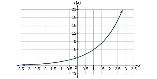
Solution

We can choose the \(y\)-intercept of the graph, \((0,3)\), as our first point. This gives us the initial value, \(a=3\). Next, choose a point on the curve some distance away from \((0,3)\) that has integer coordinates. One such point is \((2,12)\).

\[\begin{align*} y&= ab^x &&\qquad \text{Write the general form of an exponential equation}\\ y&= 3b^x &&\qquad \text{Substitute the initial value } 3 \text{ for } a\\ 12&= 3b^2 &&\qquad \text{Substitute in 12 for } y \text{ and } 2 \text{ for } x\\ 4&= b^2 &&\qquad \text{Divide by }3\\ b&= \pm 2 &&\qquad \text{Take the square root} \end{align*}\]

Because we restrict ourselves to positive values of \(b\), we will use \(b=2\). Substitute \(a\) and \(b\) into the standard form to yield the equation \(f(x)=3{(2)}^x\).

Try It \(\PageIndex{6}\)

Find an equation for the exponential function graphed in Figure \(\PageIndex{6}\).

Figure \(\PageIndex{6}\)

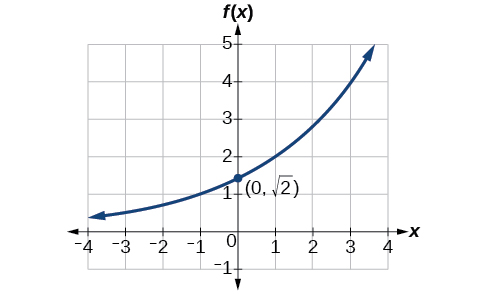
Answer

\(f(x)=\sqrt{2}{(\sqrt{2})}^x\). Answers may vary due to round-off error. The answer should be very close to \(1.4142{(1.4142)}^x\).

The Compound-Interest Formula

Savings instruments in which earnings are continually reinvested, such as mutual funds and retirement accounts, use compound interest. The term compounding refers to interest earned not only on the original value, but on the accumulated value of the account.

The annual percentage rate (APR) of an account, also called the nominal rate, is the yearly interest rate earned by an investment account. The term nominal is used when the compounding occurs a number of times other than once per year. In fact, when interest is compounded more than once a year, the effective interest rate ends up being greater than the nominal rate! This is a powerful tool for investing.

We can calculate the compound interest using the compound interest formula, which is an exponential function of the variables time \(t\), principal \(P\), yearly interest rate \(r\), and number of compounding periods in a year \(n\):

\[A(t)=P{\left (1+\dfrac{r}{n} \right )}^{nt} \nonumber\]

For example, observe Table \(\PageIndex{4}\), which shows the result of investing \($1,000\) at \(10\%\) for one year. Notice how the value of the account increases as the compounding frequency increases.

Table \(\PageIndex{4}\)

Frequency	Value after \(1\) year	(effective interest rate)
Annually	\($1100\)	\(10\%\)
Semiannually	\($1102.50\)	\(10.250\%\)
Quarterly	\($1103.81\)	\(10.381\%\)
Monthly	\($1104.71\)	\(10.471\%\)
Daily	\($1105.16\)	\(10.516\%\)

Definition: THE COMPOUND INTEREST FORMULA

Compound interest can be calculated using the formula

\[A(t)=P{\left (1+\dfrac{r}{n} \right )}^{nt} \]

where

• \(A(t)\) is the current value of the account,
• \(t\) is measured in years,
• \(P\) is the starting amount of the account, often called the principal, or more generally present value,
• \(r\) is the yearly interest rate expressed as a decimal, often called APR or nominal rate, and
• \(n\) is the number of compounding periods in one year.

Example \(\PageIndex{7}\): Calculate Compound Interest

If we invest \($3,000\) in an investment account paying \(3\%\) interest compounded quarterly, how much will the account be worth in \(10\) years?

Solution

Because we are starting with \($3,000\), \(P=3000\). Our interest rate is \(3\%\), so \(r = 0.03\). Because we are compounding quarterly, we are compounding \(4\) times per year, so \(n=4\). We want to know the value of the account in \(10\) years, so we are looking for \(A(10)\), the value when \(t = 10\).

\[\begin{align*} A(t)&= P{\left (1+\dfrac{r}{n} \right )}^{nt} \qquad \qquad \qquad \text{Use the compound interest formula}\\ A(10)&= 3000{\left (1+\dfrac{0.03}{4} \right )}^{(4)\cdot (10)} \qquad \text{Substitute using given values}\\ &\approx \$4045.05 \qquad \qquad \qquad \qquad \text{Round to two decimal places} \end{align*}\]

The account will be worth about \($4,045.05 \)  in \(10\) years.

Try It \(\PageIndex{7}\)

An initial investment of \($100,000\) at \(12\%\) interest is compounded weekly (use \(52\) weeks in a year). What will the investment be worth in \(30\) years?

Answer

about \($3,644,675.88\)

Example \(\PageIndex{8}\): Use the Compound Interest Formula to Solve for the Principal

A 529 Plan is a college-savings plan that allows relatives to invest money to pay for a child’s future college tuition; the account grows tax-free. Lily wants to set up a 529 account for her new granddaughter and wants the account to grow to \($40,000\) over \(18\) years. She believes the account will earn \(6\%\) compounded semi-annually (twice a year). To the nearest dollar, how much will Lily need to invest in the account now?

Solution

The nominal interest rate is \(6\%\), so \(r=0.06\). Interest is compounded twice a year, so \(k=2\).

We want to find the initial investment, \(P\), needed so that the value of the account will be worth \($40,000\) in \(18\) years. Substitute the given values into the compound interest formula, and solve for \(P\).

\[\begin{align*} A(t)&= P{\left (1+\dfrac{r}{n} \right )}^{nt} && \qquad \text{Use the compound interest formula}\\ 40,000&= P{\left (1+\dfrac{0.06}{2} \right )}^{2(18)} &&\qquad \text{Substitute using given values } A, r, n, t\\ 40,000&= P{(1.03)}^{36} && \qquad \text{Simplify}\\ \dfrac{40,000}{ {(1.03)}^{36} }&= P &&\qquad \text{Isolate } P\\ P&\approx \$13,801 &&\qquad \text{Divide and round to the nearest dollar} \end{align*}\]

Lily will need to invest \($13,801\) to have \($40,000\) in \(18\) years.

Try It \(\PageIndex{8}\)

In Example \(\PageIndex{9}\), how much, to the nearest dollar, would Lily need to invest if the account is compounded quarterly?

Answer

\($13,693\)

The Constant \(e\)

As we saw earlier, the amount earned on an account increases as the compounding frequency increases. Table \(\PageIndex{5}\) shows that the increase from annual to semi-annual compounding is larger than the increase from monthly to daily compounding. This might lead us to ask whether this pattern will continue.

Examine the value of \($1\) invested at \(100\%\) interest for \(1\) year, compounded at various frequencies, listed in Table \(\PageIndex{5}\).

Table \(\PageIndex{5}\)

Frequency	\(A(t)={\left (1+\dfrac{1}{n} \right )}^n\)	Value
Annually	\({\left (1+\dfrac{1}{1} \right )}^1\)	\($2\)
Semiannually	\({\left (1+\dfrac{1}{2} \right )}^2\)	\($2.25\)
Quarterly	\({\left (1+\dfrac{1}{4} \right )}^4\)	\($2.441406\)
Monthly	\({\left (1+\dfrac{1}{12} \right )}^{12}\)	\($2.613035\)
Daily	\({\left (1+\dfrac{1}{365} \right )}^{365}\)	\($2.714567\)
Hourly	\({\left (1+\dfrac{1}{8760} \right )}^{8760}\)	\($2.718127\)
Once per minute	\({\left (1+\dfrac{1}{525600} \right )}^{525600}\)	\($2.718279\)
Once per second	\({\left (1+\dfrac{1}{31536000} \right )}^{31536000}\)	\($2.718282\)

These values appear to be approaching a limit as \(n\) increases without bound. In fact, as \(n\) gets larger and larger, the expression \({\left (1+\dfrac{1}{n} \right )}^n\) approaches a number used so frequently in mathematics that it has its own name: the letter \(e\). This value is an irrational number, which means that its decimal expansion goes on forever without repeating. Its approximation to six decimal places is \(e≈2.718282\).

Definition: THE CONSTANT \(e\)

The letter \(e\) represents an irrational number

\(e = {\left (1+\dfrac{1}{n} \right )}^n \quad \text{as } n \text{ increases without bound} \)

The letter \(e\) is used as a base for many real-world exponential models. To work with base \(e\), we use the approximation, \(e≈2.718282\). The constant was named by the Swiss mathematician Leonhard Euler (1707–1783) who first investigated and discovered many of its properties.

Example \(\PageIndex{9}\): Use a Calculator to Find Powers of \(e\)

Calculate \(e^{3.14}\). Round to five decimal places.

Solution

On a calculator, press the button labeled \([e^x]\). The window shows \([e {}^( ]\). Type \(3.14\) and then close parenthesis, \([)]\). Press [ENTER]. Rounding to \(5\) decimal places, \(e^{3.14}≈23.10387\). Caution: Many scientific calculators have an “Exp” button, which is used to enter numbers in scientific notation. It is not used to find powers of \(e\).

Try It \(\PageIndex{9}\)

Use a calculator to find \(e^{−0.5}\). Round to five decimal places.

Answer

\(e^{−0.5}≈0.60653\)

Continuous Growth or Decay

So far we have worked with rational bases for exponential functions. For most real-world phenomena, however, \(e\) is used as the base for exponential functions. Exponential models that use \(e\) as the base are called continuous growth or decay models. We see these models in finance, computer science, and most of the sciences, such as physics, toxicology, and fluid dynamics.

Definition: THE CONTINUOUS GROWTH/DECAY FORMULA

For all real numbers \(t\), \(a\) and \(r\), continuous growth or decay is represented by the formula

\[A(t)=ae^{rt}\]

where

• \(a\) is the initial value,
• \(r\) is the continuous growth rate per unit time,
• \(t\) is the elapsed time.

If \(r>0\) , then the formula represents continuous growth. If \(r<0\), then the formula represents continuous decay.

For business applications, the continuous growth formula is called the continuous compounding formula and takes the form

\[A(t)=Pe^{rt}\]

where

• \(P\) is the principal or the initial amount invested,
• \(r\) is the growth or interest rate per unit time,
• \(t\) is the period or term of the investment.

 How to: Construct and evaluate a continuous growth or decay function \(A(t) = a e^{rt} \)

1. Use the information in the problem to determine \(a\), the initial value of the function.
2. Use the information in the problem to determine the growth rate \(r\).
   • If the problem refers to continuous growth, then \(r>0\).
   • If the problem refers to continuous decay, then \(r<0\).
3. Use the information in the problem to determine the time \(t\).
4. Substitute the given information into the continuous growth formula and evaluate \(A(t)\).

Example \(\PageIndex{10}\): Calculate Continuous Growth

A person invested \($1,000\) in an account earning a nominal \(10\%\) per year compounded continuously. How much was in the account at the end of one year?

Solution

Since the account is growing in value, this is a continuous compounding problem with growth rate \(r=0.10\). The initial investment was \($1,000\), so \(P=1000\). We use the continuous compounding formula to find the value after \(t=1\) year:

\[\begin{align*} A(t)&= Pe^{rt} &&\qquad \text{Use the continuous compounding formula}\\ &= 1000{(e)}^{0.1} &&\qquad \text{Substitute known values for } P, r, t\\ &\approx 1105.17 &&\qquad \text{Use a calculator to approximate} \end{align*}\]

The account is worth \($1,105.17\) after one year.

Try It \(\PageIndex{10}\)

A person invests \($100,000\) at a nominal \(12\%\) interest per year compounded continuously. What will be the value of the investment in \(30\) years?

Answer

\($3,659,823.44\)

Example \(\PageIndex{11}\): Calculate Continuous Decay

Radon-222 decays at a continuous rate of \(17.3\%\) per day. How much will \(100\) mg of Radon-222 decay to in \(3\) days?

Solution

Since the substance is decaying, the rate, \(17.3\%\), is negative. So, \(r = −0.173\). The initial amount of Radon-222 was \(100\) mg, so \(a=100\). We use the continuous decay formula to find the value after \(t=3\) days:

\[\begin{align*} A(t)&= ae^{rt} &&\qquad \text{Use the continuous growth formula}\\ &= 100e^{-0.173(3)} &&\qquad \text{Substitute known values for } a, r, t\\ &\approx 59.5115 &&\qquad \text{Use a calculator to approximate} \end{align*}\]

So \(59.5115\) mg of Radon-222 will remain.

Try It \(\PageIndex{11}\)

Using the data in Example \(\PageIndex{12}\), how much Radon-222 will remain after one year?

Answer

\(3.77E-26\) (This is calculator notation for the number written as \(3.77×10^{−26}\) in scientific notation. While the output of an exponential function is never zero, this number is so close to zero that for all practical purposes we can accept zero as the answer.)

Key Equations

definition of the exponential function	\(f(x)=b^x\), where \(b>0\), \(b≠1\)
definition of exponential growth/decay	\(f(x)=ab^x\), where  \(b>0\), \(b≠1\)
compound interest formula	\(A(t)=P{(1+\dfrac{r}{n})}^{nt}\) , where \(A(t)\) is the account value at time \(t\) \(t\) is the number of years \(P\) is the initial investment, often called the principal \(r\) is the annual percentage rate (APR), or nominal rate \(n\) is the number of compounding periods in one year
continuous growth formula	\(A(t)=ae^{rt}\), where \(t\) is the number of unit time periods of growth \(a\) is the starting amount (in the continuous compounding formula a is replaced with \(P\), the principal) \(e\) is the mathematical constant, \(e≈2.718282\)

Key Concepts

• An exponential function is defined as a function with a positive constant other than \(1\) raised to a variable exponent. 
• An exponential model can be found when the growth rate and initial value are known. 
• An exponential model can be found when the two data points from the model are known. 
• An exponential model can be found using two data points from the graph of the model. 
• The value of an account at any time \(t\) can be calculated using the compound interest formula when the principal, annual interest rate, and compounding periods are known. 
• The initial investment of an account can be found using the compound interest formula when the value of the account, annual interest rate, compounding periods, and life span of the account are known. 
• The number \(e\) is a mathematical constant often used as the base of real world exponential growth and decay models. Its decimal approximation is \(e≈2.718282\).
• Scientific and graphing calculators have the key \([e^x]\) or \([exp(x)]\) for calculating powers of \(e\). 
• Continuous growth or decay models are exponential models that use \(e\) as the base. Continuous growth and decay models can be found when the initial value and growth or decay rate are known. 

Contributors

• Jay Abramson (Arizona State University) with contributing authors. Textbook content produced by OpenStax College is licensed under a Creative Commons Attribution License 4.0 license. Download for free at https://openstax.org/details/books/precalculus.