
13.6: Directional Derivatives and the Gradient
- Page ID
- 10954

In Partial Derivatives, we introduced the partial derivative. A function \(z=f(x,y)\) has two partial derivatives: \(∂z/∂x\) and \(∂z/∂y\). These derivatives correspond to each of the independent variables and can be interpreted as instantaneous rates of change (that is, as slopes of a tangent line). For example, \(∂z/∂x\) represents the slope of a tangent line passing through a given point on the surface defined by \(z=f(x,y),\) assuming the tangent line is parallel to the \(x\)-axis. Similarly, \(∂z/∂y\) represents the slope of the tangent line parallel to the \(y\)-axis. Now we consider the possibility of a tangent line parallel to neither axis.
Directional Derivatives
We start with the graph of a surface defined by the equation \(z=f(x,y)\). Given a point \((a,b)\) in the domain of \(f\), we choose a direction to travel from that point. We measure the direction using an angle \(θ\), which is measured counterclockwise in the \(xy\)-plane, starting at zero from the positive \(x\)-axis (Figure \(\PageIndex{1}\)). The distance we travel is \(h\) and the direction we travel is given by the unit vector \(\vecs u=(\cos θ)\,\hat{\mathbf i}+(\sin θ)\,\hat{\mathbf j}.\) Therefore, the \(z\)-coordinate of the second point on the graph is given by \(z=f(a+h\cos θ,b+h\sin θ).\)

We can calculate the slope of the secant line by dividing the difference in \(z\)-values by the length of the line segment connecting the two points in the domain. The length of the line segment is \(h\). Therefore, the slope of the secant line is
\[m_{sec}=\dfrac{f(a+h\cos θ,b+h\sin θ)−f(a,b)}{h}\]
To find the slope of the tangent line in the same direction, we take the limit as \(h\) approaches zero.
Definition: Directional Derivatives
Suppose \(z=f(x,y)\) is a function of two variables with a domain of \(D\). Let \((a,b)∈D\) and define \(\vecs u=(\cos θ)\,\hat{\mathbf i}+(\sin θ)\,\hat{\mathbf j}\). Then the directional derivative of \(f\) in the direction of \(\vecs u\) is given by
\[D_{\vecs u}f(a,b)=\lim_{h→0}\dfrac{f(a+h \cos θ,b+h\sin θ)−f(a,b)}{h} \label{DD}\]
provided the limit exists.
Equation \ref{DD} provides a formal definition of the directional derivative that can be used in many cases to calculate a directional derivative.
Note that since the point \((a, b)\) is chosen randomly from the domain \(D\) of the function \(f\), we can use this definition to find the directional derivative as a function of \(x\) and \(y\).
That is,
\[D_{\vecs u}f(x,y)=\lim_{h→0}\dfrac{f(x+h \cos θ,y+h\sin θ)−f(x,y)}{h} \label{DDxy}\]
Example \(\PageIndex{1}\): Finding a Directional Derivative from the Definition
Let \(θ=\arccos(3/5).\) Find the directional derivative \(D_{\vecs u}f(x,y)\) of \(f(x,y)=x^2−xy+3y^2\) in the direction of \(\vecs u=(\cos θ)\,\hat{\mathbf i}+(\sin θ)\,\hat{\mathbf j}\).
Then determine \(D_{\vecs u}f(−1,2)\).
Solution
First of all, since \(\cos θ=3/5\) and \(θ\) is acute, this implies
\[\sin θ=\sqrt{1−\left(\dfrac{3}{5}\right)^2}=\sqrt{\dfrac{16}{25}}=\dfrac{4}{5}. \nonumber\]
Using \(f(x,y)=x^2−xy+3y^2,\) we first calculate \(f(x+h\cos θ,y+h\sin θ)\):
\[\begin{align*} f(x+h\cos θ,y+h\sin θ)&=(x+h\cos θ)^2−(x+h\cos θ)(y+h\sin θ)+3(y+h\sin θ)^2 \\&=x^2+2xh\cos θ+h^2\cos^2 θ−xy−xh\sin θ−yh\cos θ−h^2\sin θ\cos θ+3y^2+6yh\sin θ+3h^2\sin^2 θ \\ &=x^2+2xh(\dfrac{3}{5})+\dfrac{9h^2}{25}−xy−\dfrac{4xh}{5}−\dfrac{3yh}{5}−\dfrac{12h^2}{25}+3y^2+6yh(\dfrac{4}{5})+3h^2(\dfrac{16}{25})\\&=x^2−xy+3y^2+\dfrac{2xh}{5}+\dfrac{9h^2}{5}+\dfrac{21yh}{5}. \end{align*}\]
We substitute this expression into Equation \ref{DD} with \(a = x\) and \(b = y\):
\[\begin{align*} D_{\vecs u}f(x,y)&=\lim_{h→0}\dfrac{f(x+h\cos θ,y+h\sin θ)−f(x,y)}{h}\\ &=\lim_{h→0}\dfrac{(x^2−xy+3y^2+\dfrac{2xh}{5}+\dfrac{9h^2}{5}+\dfrac{21yh}{5})−(x^2−xy+3y^2)}{h}\\ &=\lim_{h→0}\dfrac{\dfrac{2xh}{5}+\dfrac{9h^2}{5}+\dfrac{21yh}{5}}{h}\\ &=\lim_{h→0}\dfrac{2x}{5}+\dfrac{9h}{5}+\dfrac{21y}{5}\\&=\dfrac{2x+21y}{5}. \end{align*}\]
To calculate \(D_{\vecs u}f(−1,2),\) we substitute \(x=−1\) and \(y=2\) into this answer (Figure \(\PageIndex{2}\)):
\[ D_{\vecs u}f(−1,2)=\dfrac{2(−1)+21(2)}{5}=\dfrac{−2+42}{5}=8. \nonumber\]

An easier approach to calculating directional derivatives that involves partial derivatives is outlined in the following theorem.
Directional Derivative of a Function of Two Variables
Let \(z=f(x,y)\) be a function of two variables \(x\) and \(y\), and assume that \(f_x\) and \(f_y\) exist. Then the directional derivative of \(f\) in the direction of \(\vecs u=(\cos θ)\,\hat{\mathbf i}+(\sin θ)\,\hat{\mathbf j}\) is given by
\[D_{\vecs u}f(x,y)=f_x(x,y)\cos θ+f_y(x,y)\sin θ. \label{DD2v}\]
Proof
Applying the definition of a directional derivative stated above in Equation \ref{DD}, the directional derivative of \(f\) in the direction of \(\vecs u=(\cos θ)\,\hat{\mathbf i}+(\sin θ)\,\hat{\mathbf j}\) at a point \((x_0, y_0)\) in the domain of \(f\) can be written
\[D_{\vecs u}f((x_0, y_0))=\lim_{t→0}\dfrac{f(x_0+t \cos θ,y_0+t\sin θ)−f(x_0,y_0)}{t}.\]
Let \(x=x_0+t\cos θ\) and \(y=y_0+t\sin θ,\) and define \(g(t)=f(x,y)\). Since \(f_x\) and \(f_y\) both exist, we can use the chain rule for functions of two variables to calculate \(g′(t)\):
\[g′(t)=\dfrac{∂f}{∂x}\dfrac{dx}{dt}+\dfrac{∂f}{∂y}\dfrac{dy}{dt}=f_x(x,y)\cos θ+f_y(x,y)\sin θ.\]
If \(t=0,\) then \(x=x_0\) and \(y=y_0,\) so
\[g′(0)=f_x(x_0,y_0)\cos θ+f_y(x_0,y_0)\sin θ\]
By the definition of \(g′(t),\) it is also true that
\[g′(0)=\lim_{t→0}\dfrac{g(t)−g(0)}{t}=\lim_{t→0}\dfrac{f(x_0+t\cos θ,y_0+t\sin θ)−f(x_0,y_0)}{t}.\]
Therefore, \(D_{\vecs u}f(x_0,y_0)=f_x(x_0,y_0)\cos θ+f_y(x_0,y_0)\sin θ\).
Since the point \( (x_0,y_0) \) is an arbitrary point from the domain of \(f\), this result holds for all points in the domain of \(f\) for which the partials \(f_x\) and \(f_y\) exist.
Therefore, \[D_{\vecs u}f(x,y)=f_x(x,y)\cos θ+f_y(x,y)\sin θ.\]
□
Example \(\PageIndex{2}\): Finding a Directional Derivative: Alternative Method
Let \(θ=\arccos (3/5).\) Find the directional derivative \(D_{\vecs u}f(x,y)\) of \(f(x,y)=x^2−xy+3y^2\) in the direction of \(\vecs u=(\cos θ)\,\hat{\mathbf i}+(\sin θ)\,\hat{\mathbf j}\).
Then determine \(D_{\vecs u}f(−1,2)\).
Solution
First, we must calculate the partial derivatives of \(f\):
\[\begin{align*}f_x(x,y)&=2x−y \\ f_y(x,y)&=−x+6y, \end{align*}\]
Then we use Equation \ref{DD2v} with \(θ=\arccos (3/5)\):
\[\begin{align*} D_{\vecs u}f(x,y)&=f_x(x,y)\cos θ+f_y(x,y)\sin θ \\&=(2x−y)\dfrac{3}{5}+(−x+6y)\dfrac{4}{5} \\ &=\dfrac{6x}{5}−\dfrac{3y}{5}−\dfrac{4x}{5}+\dfrac{24y}{5}\\&=\dfrac{2x+21y}{5}. \end{align*}\]
To calculate \(D_{\vecs u}f(−1,2),\) let \(x=−1\) and \(y=2\):
\[D_{\vecs u}f(−1,2)=\dfrac{2(−1)+21(2)}{5}=\dfrac{−2+42}{5}=8.\]
This is the same answer obtained in Example \(\PageIndex{1}\).
Exercise \(\PageIndex{1}\):
Find the directional derivative \(D_{\vecs u}f(x,y)\) of \(f(x,y)=3x^2y−4xy^3+3y^2−4x\) in the direction of \(\vecs u=(\cos \dfrac{π}{3})\,\hat{\mathbf i}+(\sin \dfrac{π}{3})\,\hat{\mathbf j}\) using Equation \ref{DD2v}.
What is \(D_{\vecs u} f(3,4)\)?
- Hint
-
Calculate the partial derivatives and determine the value of \(θ\).
- Answer
-
\(D_{\vecs u}f(x,y)=\dfrac{(6xy−4y^3−4)(1)}{2}+\dfrac{(3x^2−12xy^2+6y)\sqrt{3}}{2}\)
\(D_{\vecs u}f(3,4)=\dfrac{72−256−4}{2}+\dfrac{(27−576+24)\sqrt{3}}{2}=−94−\dfrac{525\sqrt{3}}{2}\)
If the vector that is given for the direction of the derivative is not a unit vector, then it is only necessary to divide by the norm of the vector. For example, if we wished to find the directional derivative of the function in Example \(\PageIndex{2}\) in the direction of the vector \(⟨−5,12⟩\), we would first divide by its magnitude to get \(\vecs u\). This gives us \(\vecs u=⟨−\frac{5}{13},\frac{12}{13}⟩\).
Then
\[ \begin{align*} D_{\vecs u}f(x,y)&=f_x(x,y)\cos θ+f_y(x,y)\sin θ \\ &=−\dfrac{5}{13}(2x−y)+\dfrac{12}{13}(−x+6y) \\ &=−\dfrac{22}{13}x+\dfrac{17}{13}y \end{align*}\]
Gradient
The right-hand side of Equation \ref{DD2v} is equal to \(f_x(x,y)\cos θ+f_y(x,y)\sin θ,\) which can be written as the dot product of two vectors. Define the first vector as \(\vecs ∇f(x,y)=f_x(x,y)\,\hat{\mathbf i}+f_y(x,y)\,\hat{\mathbf j}\) and the second vector as \(\vecs u=(\cos θ)\,\hat{\mathbf i}+(\sin θ)\,\hat{\mathbf j}\). Then the right-hand side of the equation can be written as the dot product of these two vectors:
\[D_{\vecs u}f(x,y)=\vecs ∇f(x,y)⋅\vecs u. \label{gradDirDer}\]
The first vector in Equation \ref{gradDirDer} has a special name: the gradient of the function \(f\). The symbol \(∇\) is called nabla and the vector \(\vecs ∇f\) is read “del \(f\).”
Definition: The Gradient
Let \(z=f(x,y)\) be a function of \(x\) and \(y\) such that \(f_x\) and \(f_y\) exist. The vector \(\vecs ∇f(x,y)\) is called the gradient of \(f\) and is defined as
\[\vecs ∇f(x,y)=f_x(x,y)\,\hat{\mathbf i}+f_y(x,y)\,\hat{\mathbf j}. \label{grad}\]
The vector \(\vecs ∇f(x,y)\) is also written as “grad \(f\).”
Example \(\PageIndex{3}\): Finding Gradients
Find the gradient \(\vecs ∇f(x,y)\) of each of the following functions:
- \(f(x,y)=x^2−xy+3y^2\)
- \(f(x,y)=\sin 3 x \cos 3y\)
Solution
For both parts a. and b., we first calculate the partial derivatives \(f_x\) and \(f_y\), then use Equation \ref{grad}.
a. \( f_x(x,y)=2x−y\) and \(f_y(x,y)=−x+6y\), so
\[\begin{align*} \vecs ∇f(x,y)&=f_x(x,y)\,\hat{\mathbf i}+f_y(x,y)\,\hat{\mathbf j}\\&=(2x−y)\,\hat{\mathbf i}+(−x+6y)\,\hat{\mathbf j}.\end{align*}\]
b. \( f_x(x,y)=3\cos 3x \cos 3y\) and \(f_y(x,y)=−3\sin 3x \sin 3y\), so
\[\begin{align*} \vecs ∇f(x,y)&=f_x(x,y)\,\hat{\mathbf i}+f_y(x,y)\,\hat{\mathbf j} \\ &=(3\cos 3x \cos 3y)\,\hat{\mathbf i}−(3\sin 3x \sin 3y)\,\hat{\mathbf j}. \end{align*}\]
Exercise \(\PageIndex{2}\)
Find the gradient \(\vecs ∇f(x,y)\) of \(f(x,y)=\dfrac{x^2−3y^2}{2x+y}\).
- Hint
-
Calculate the partial derivatives, then use Equation \ref{grad}.
- Answer
-
\(\vecs ∇f(x,y)=\dfrac{2x^2+2xy+6y^2}{(2x+y)^2}\,\hat{\mathbf i}−\dfrac{x^2+12xy+3y^2}{(2x+y)^2}\,\hat{\mathbf j}\)
The gradient has some important properties. We have already seen one formula that uses the gradient: the formula for the directional derivative. Recall from The Dot Product that if the angle between two vectors \(\vecs a\) and \(\vecs b\) is \(φ\), then \(\vecs a⋅\vecs b=‖\vecs a‖‖\vecs b‖\cos φ.\) Therefore, if the angle between \(\vecs ∇f(x_0,y_0)\) and \(\vecs u=(cosθ)\,\hat{\mathbf i}+(sinθ)\,\hat{\mathbf j}\) is \(φ\), we have
\[D_{\vecs u}f(x_0,y_0)=\vecs ∇f(x_0,y_0)⋅\vecs u=\|\vecs ∇f(x_0,y_0)\|‖\vecs u‖\cos φ=\|\vecs ∇f(x_0,y_0)\|\cos φ.\]
The \(‖\vecs u‖\) disappears because \(\vecs u\) is a unit vector. Therefore, the directional derivative is equal to the magnitude of the gradient evaluated at \((x_0,y_0)\) multiplied by \(\cos φ\). Recall that \(\cos φ\) ranges from \(−1\) to \(1\).
If \(φ=0,\) then \(\cos φ=1\) and \(\vecs ∇f(x_0,y_0)\) and \(\vecs u\) both point in the same direction.
If \(φ=π\), then \(\cos φ=−1\) and \(\vecs ∇f(x_0,y_0)\) and \(\vecs u\) point in opposite directions.
In the first case, the value of \(D_{\vecs u}f(x_0,y_0)\) is maximized and in the second case, the value of \(D_{\vecs u}f(x_0,y_0)\) is minimized.
We can also see that if \(\vecs ∇f(x_0,y_0)=\vecs 0\), then
\[ D_{\vecs u}f(x_0,y_0)=\vecs ∇f(x_0,y_0)⋅\vecs u=0\]
for any vector \(\vecs u\). These three cases are outlined in the following theorem.
Properties of the Gradient
Suppose the function \(z=f(x,y)\) is differentiable at \((x_0,y_0)\) (Figure \(\PageIndex{3}\)).
- If \(\vecs ∇f(x_0,y_0)=\vecs 0\), then \(D_{\vecs u}f(x_0,y_0)=0\) for any unit vector \(\vecs u\).
- If \(\vecs ∇f(x_0,y_0)≠\vecs 0\), then \(D_{\vecs u}f(x_0,y_0)\) is maximized when \(\vecs u\) points in the same direction as \(\vecs ∇f(x_0,y_0)\). The maximum value of \(D_{\vecs u}f(x_0,y_0)\) is \(\|\vecs ∇f(x_0,y_0)\|\).
- If \(\vecs ∇f(x_0,y_0)≠\vecs 0\), then \(D_{\vecs u}f(x_0,y_0)\) is minimized when \(\vecs u\) points in the opposite direction from \(\vecs ∇f(x_0,y_0)\). The minimum value of \(D_{\vecs u}f(x_0,y_0)\) is \(−\|\vecs ∇f(x_0,y_0)\|\).
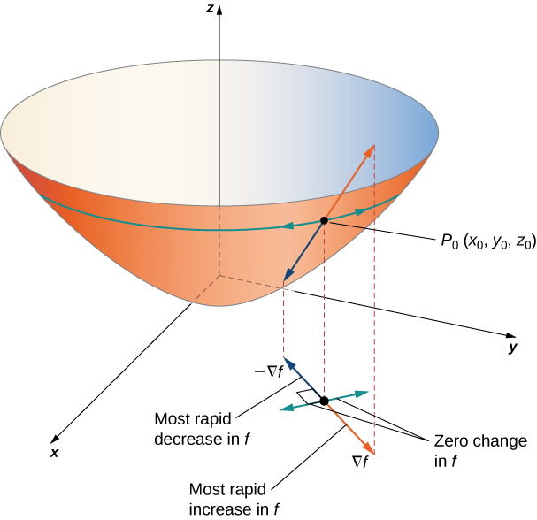
Note: Gradient indicates direction of steepest ascent
Since the gradient vector points in the direction within the domain of \(f\) that corresponds to the maximum value of the directional derivative, \(D_{\vecs u}f(x_0,y_0)\), we say that the gradient vector points in the direction of steepest ascent or most rapid increase in \(f\), that is, at any given point, the gradient points in the direction with the steepest uphill slope.
Example \(\PageIndex{4}\): Finding a Maximum Directional Derivative
Find the direction for which the directional derivative of \(f(x,y)=3x^2−4xy+2y^2\) at \((−2,3)\) is a maximum. What is the maximum value?
Solution:
The maximum value of the directional derivative occurs when \(\vecs ∇f\) and the unit vector point in the same direction. Therefore, we start by calculating \(\vecs ∇f(x,y\)):
\[f_x(x,y)=6x−4y \; \text{and}\; f_y(x,y)=−4x+4y \nonumber\]
so
\[\vecs ∇f(x,y)=f_x(x,y)\,\hat{\mathbf i}+f_y(x,y)\,\hat{\mathbf j}=(6x−4y)\,\hat{\mathbf i}+(−4x+4y)\,\hat{\mathbf j}. \nonumber\]
Next, we evaluate the gradient at \((−2,3)\):
\[\vecs ∇f(−2,3)=(6(−2)−4(3))\,\hat{\mathbf i}+(−4(−2)+4(3))\,\hat{\mathbf j}=−24\,\hat{\mathbf i}+20\,\hat{\mathbf j}. \nonumber\]
The gradient vector gives the direction of the maximum value of the directional derivative.
The maximum value of the directional derivative at \((−2,3)\) is \(\|\vecs ∇f(−2,3)\|=4\sqrt{61}\) (see the Figure \(\PageIndex{4}\)).

Exercise \(\PageIndex{3}\):
Find the direction for which the directional derivative of \(g(x,y)=4x−xy+2y^2\) at \((−2,3)\) is a maximum. What is the maximum value?
- Hint
-
Evaluate the gradient of \(g\) at point \((−2,3)\).
- Answer
-
The gradient of \(g\) at \((−2,3)\) is \(\vecs ∇g(−2,3)=\,\hat{\mathbf i}+14\,\hat{\mathbf j}\). This gives the direction of the maximum value of the directional derivative at the point \((−2,3)\).
The maximum value of the directional derivative is \(\|\vecs ∇g(−2,3)\|=\sqrt{197}\).
Figure \(\PageIndex{5}\) shows a portion of the graph of the function \(f(x,y)=3+\sin x \sin y\). Given a point \((a,b)\) in the domain of \(f\), the maximum value of the directional derivative at that point is given by \(\|\vecs ∇f(a,b)\|\). This would equal the rate of greatest ascent if the surface represented a topographical map. If we went in the opposite direction, it would be the rate of greatest descent.

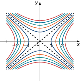
When using a topographical map, the steepest slope is always in the direction where the contour lines are closest together (Figure \(\PageIndex{6}\)). This is analogous to the contour map of a function, assuming the level curves are obtained for equally spaced values throughout the range of that function.
Gradients and Level Curves
Recall that if a curve is defined parametrically by the function pair \((x(t),y(t)),\) then the vector \(x′(t)\,\hat{\mathbf i}+y′(t)\,\hat{\mathbf j}\) is tangent to the curve for every value of \(t\) in the domain. Now let’s assume \(z=f(x,y)\) is a differentiable function of \(x\) and \(y\), and \((x_0,y_0)\) is in its domain. Let’s suppose further that \(x_0=x(t_0)\) and \(y_0=y(t_0)\) for some value of \(t\), and consider the level curve \(f(x,y)=k\). Define \(g(t)=f(x(t),y(t))\) and calculate \(g′(t)\) on the level curve. By the chain Rule,
\[g′(t)=f_x(x(t),y(t))x′(t)+f_y(x(t),y(t))y′(t).\]
But \(g′(t)=0\) because \(g(t)=k\) for all \(t\). Therefore, on the one hand,
\[f_x(x(t),y(t))x′(t)+f_y(x(t),y(t))y′(t)=0;\]
on the other hand,
\[f_x(x(t),y(t))x′(t)+f_y(x(t),y(t))y′(t)=\vecs ∇f(x,y)⋅⟨x′(t),y′(t)⟩.\]
Therefore,
\[\vecs ∇f(x,y)⋅⟨x′(t),y′(t)⟩=0.\]
Thus, the dot product of these vectors is equal to zero, which implies they are orthogonal. However, the second vector is tangent to the level curve, which implies the gradient must be normal to the level curve, which gives rise to the following theorem.
Gradient Is Normal to the Level Curve
Suppose the function \(z=f(x,y)\) has continuous first-order partial derivatives in an open disk centered at a point \((x_0,y_0)\). If \(\vecs ∇f(x_0,y_0)≠\vecs 0\), then \(\vecs ∇f(x_0,y_0)\) is normal to the level curve of \(f\) at \((x_0,y_0)\).
We can use this theorem to find tangent and normal vectors to level curves of a function.
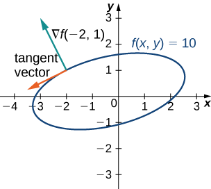
Example \(\PageIndex{5}\): Finding Tangents to Level Curves
For the function \(f(x,y)=2x^2−3xy+8y^2+2x−4y+4,\) find a tangent vector to the level curve at point \((−2,1)\). Graph the level curve corresponding to \(f(x,y)=18\) and draw in \(\vecs ∇f(−2,1)\) and a tangent vector.
Solution:
First, we must calculate \(\vecs ∇f(x,y):\)
\[f_x(x,y)=4x−3y+2 \;\text{and}\; f_y=−3x+16y−4 \;\text{so}\; \vecs ∇f(x,y)=(4x−3y+2)\,\hat{\mathbf i}+(−3x+16y−4)\,\hat{\mathbf j}.\]
Next, we evaluate \(\vecs ∇f(x,y)\) at \((−2,1):\)
\[\vecs ∇f(−2,1)=(4(−2)−3(1)+2)\,\hat{\mathbf i}+(−3(−2)+16(1)−4)\,\hat{\mathbf j}=−9\,\hat{\mathbf i}+18\,\hat{\mathbf j}.\]
This vector is orthogonal to the curve at point \((−2,1)\). We can obtain a tangent vector by reversing the components and multiplying either one by \(−1\). Thus, for example, \(−18\,\hat{\mathbf i}−9\,\hat{\mathbf j}\) is a tangent vector (see the following graph).
Exercise \(\PageIndex{4}\):
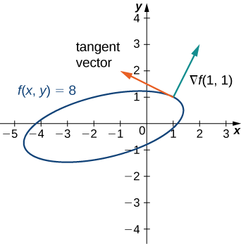
For the function \(f(x,y)=x^2−2xy+5y^2+3x−2y+3\), find the tangent to the level curve at point \((1,1)\). Draw the graph of the level curve corresponding to \(f(x,y)=8\) and draw \(\vecs ∇f(1,1)\) and a tangent vector.
- Hint
-
Calculate the gradient at point \((1,1)\).
- Answer
-
\(\vecs ∇f(x,y)=(2x−2y+3)\,\hat{\mathbf i}+(−2x+10y−2)\,\hat{\mathbf j}\)
\(\vecs ∇f(1,1)=3\,\hat{\mathbf i}+6\,\hat{\mathbf j}\)
Tangent vector: \(6\,\hat{\mathbf i}−3\,\hat{\mathbf j}\) or \(−6\,\hat{\mathbf i}+3\,\hat{\mathbf j}\)
The fact that the gradient of a surface always points in the direction of steepest increase/decrease is very useful, as illustrated in the following example.
Example \(\PageIndex{6}\): The flow of water downhill
Consider the surface given by \(f(x,y)= 20-x^2-2y^2\). Water is poured on the surface at \((1,\frac{1}{4})\). What path does it take as it flows downhill?
SOLUTION
Let \(\vecs r (t) = \langle x(t), y(t)\rangle\) be the vector--valued function describing the path of the water in the \(xy\)-plane; we seek \(x(t)\) and \(y(t)\). We know that water will always flow downhill in the steepest direction; therefore, at any point on its path, it will be moving in the direction of \(-\vecs\nabla f\). (We ignore the physical effects of momentum on the water.) Thus \(\vecs r '(t)\) will be parallel to \(\vecs\nabla f\), and there is some constant \(c\) such that \(c\vecs\nabla f(t) = \vec r '(t) = \langle x'(t), y'(t)\rangle\).
We find \(\vecs\nabla f(x,y) = \langle -2x, -4y\rangle\) and write \(x'(t)\) as \(\frac{dx}{dt}\) and \(y'(t)\) as \(\frac{dy}{dt}\). Then
\[\begin{align*}
c\vecs\nabla f(t) &= \langle x'(t), y'(t)\rangle \\
\langle -2cx, -4cy \rangle & = \langle \frac{dx}{dt}, \frac{dy}{dt}\rangle.
\end{align*}\]
This implies
\[-2cx = \frac{dx}{dt} \quad \text{and} \quad -4cy =\frac{dy}{dt}, \text{ i.e.,}\]
\[c = -\frac{1}{2x}\frac{dx}{dt} \quad \text{and} \quad c =-\frac{1}{4y}\frac{dy}{dt}.\]
As \(c\) equals both expressions, we have
\[\frac{1}{4y}\frac{dy}{dt} = \frac{1}{2x}\frac{dx}{dt}.\]
To find an explicit relationship between \(x\) and \(y\), we can integrate both sides with respect to \(t\). Recall from our study of differentials that \( \frac{dx}{dt}dt = dx\). Thus:
\[\begin{align*}
\int \frac{1}{4y}\frac{dy}{dt}\ dt &= \int \frac{1}{2x}\frac{dx}{dt}\ dt \\
\int\frac{1}{4y}\ dy &= \int \frac{1}{2x}\ dx \\
\frac14\ln|y| &= \frac 12\ln|x| +C_1\\
\ln|y| &= 2\ln|x| +C_1\\
\ln|y| &= \ln |x^2|+C_1 \end{align*}\]
Now raise both sides as a power of \(e\):
\[\begin{align*}
|y| &= e^{\ln |x^2|+C_1}\\
|y| &= e^{\ln x^2}e^{C_1}\\
y &= \pm e^{C_1}x^2
\end{align*}\]
Then \[ y = Cx^2, \quad \text{where}\; C = \pm e^{C_1} \; \text{or} \; C = 0.\]
As the water started at the point \((1,\frac{1}{4})\), we can now solve for \(C\):
\[C(1)^2 = \frac14 \quad \Rightarrow \quad C = \frac14.\]
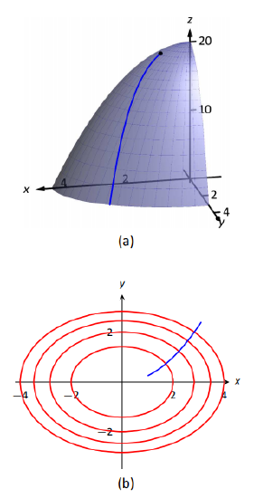
Figure \(\PageIndex{8}\): A graph of the surface along with the path in the \(xy\)-plane with the level curves.
Thus the water follows the curve \(y=\frac{x^2}{4}\) in the \(xy\)-plane. The surface and the path of the water is graphed in Figure \(\PageIndex{8}\). In part (b) of the figure, the level curves of the surface are plotted in the \(xy\)-plane, along with the curve \(y=\frac{x^2}{4}\). Notice how the path intersects the level curves at right angles. As the path follows the gradient downhill, this reinforces the fact that the gradient is orthogonal to level curves.
Three-Dimensional Gradients and Directional Derivatives
The definition of a gradient can be extended to functions of more than two variables.
Definition: Gradients in 3D
Let \(w=f(x, y, z)\) be a function of three variables such that \(f_x, \, f_y\), and \(f_z\) exist. The vector \(\vecs ∇ f(x,y,z)\) is called the gradient of \(f\) and is defined as
\[\vecs ∇f(x,y,z)=f_x(x,y,z)\,\hat{\mathbf i}+f_y(x,y,z)\,\hat{\mathbf j}+f_z(x,y,z)\,\hat{\mathbf k}.\label{grad3d}\]
\(\vecs ∇f(x,y,z)\) can also be written as grad \(f(x,y,z).\)
Calculating the gradient of a function in three variables is very similar to calculating the gradient of a function in two variables. First, we calculate the partial derivatives \(f_x, \, f_y,\) and \(f_z\), and then we use Equation \ref{grad3d}.
Example \(\PageIndex{7}\): Finding Gradients in Three Dimensions
Find the gradient \(\vecs ∇f(x,y,z)\) of each of the following functions:
- \(f(x,y,z)=5x^2−2xy+y^2−4yz+z^2+3xz\)
- \(f(x,y,z)=e^{−2z}\sin 2x \cos 2y\)
Solution:
For both parts a. and b., we first calculate the partial derivatives \(f_x,f_y,\) and \(f_z\), then use Equation \ref{grad3d}.
a. \(f_x(x,y,z)=10x−2y+3z\), \(f_y(x,y,z)=−2x+2y−4z\), and \( f_z(x,y,z)=3x−4y+2z\), so
\[\begin{align*} \vecs ∇f(x,y,z)&=f_x(x,y,z)\,\hat{\mathbf i}+f_y(x,y,z)\,\hat{\mathbf j}+f_z(x,y,z)\,\hat{\mathbf k} \\ &=(10x−2y+3z)\,\hat{\mathbf i}+(−2x+2y−4z)\,\hat{\mathbf j}+(3x-4y+2z)\,\hat{\mathbf k}. \end{align*}\]
b. \(f_x(x,y,z) =2e^{−2z}\cos 2x \cos 2y\), \( f_y(x,y,z)=−2e^{−2z} \sin 2x \sin 2y\), and \(f_z(x,y,z)=−2e^{−2z}\sin 2x \cos 2y\), so
\[\begin{align*} \vecs ∇f(x,y,z)&=f_x(x,y,z)\,\hat{\mathbf i}+f_y(x,y,z)\,\hat{\mathbf j}+f_z(x,y,z)\,\hat{\mathbf k} \\&=(2e^{−2z}\cos 2x \cos 2y)\,\hat{\mathbf i}+(−2e^{−2z}\sin 2x \sin 2y)\,\hat{\mathbf j}+(−2e^{−2z}\sin 2x \cos 2y)\,\hat{\mathbf k} \\ & =2e^{−2z}(\cos 2x \cos 2y \,\hat{\mathbf i}−\sin 2x \sin 2y\,\hat{\mathbf j}−\sin 2x \cos 2y\,\hat{\mathbf k}). \end{align*}\]
Exercise \(\PageIndex{5}\):
Find the gradient \(\vecs ∇f(x,y,z)\) of \(f(x,y,z)=\dfrac{x^2−3y^2+z^2}{2}\) and find its gradient vector at the point \( (-1, 2, 3) \).
- Answer
-
\(\vecs ∇f(x,y,z)=x\,\hat{\mathbf i}−3y\,\hat{\mathbf j}+z\,\hat{\mathbf k}\)
\(\vecs ∇f(-1,2,3)=-\hat{\mathbf i}−6\,\hat{\mathbf j}+3\,\hat{\mathbf k}\)
the gradient of a function of three variables is normal to the level surface
Suppose the function \(z=f(x,y,z)\) has continuous first-order partial derivatives in an open sphere centered at a point \((x_0,y_0,z_0)\). If \(\vecs ∇f(x_0,y_0,z_0)≠\vecs 0\), then \(\vecs ∇f(x_0,y_0,z_0)\) is normal to the level surface of \(f\) at \((x_0,y_0,z_0)\).
Figure \(\PageIndex{9}\) shows the gradient vectors at various points on a level surface of the function in Exercise \(\PageIndex{5}\). The points shown on the level surface are: \( (-1, 2, 3) \), \( (3, -2, -1) \), \( (0, \sqrt{\frac{2}{3}}, 0) \), \( (2, \sqrt{\frac{10}{3}}, 2) \), and \( (2, \sqrt{\frac{10}{3}}, -2) \).
Figure \(\PageIndex{9}\): A level surface of the function \(f(x,y,z)=\dfrac{x^2−3y^2+z^2}{2}\) for \(C = -1\) along with various points on this level surface and the corresponding gradient vectors. Note how these gradient vectors are normal to this level surface.
The directional derivative can also be generalized to functions of three variables. To determine a direction in three dimensions, a vector with three components is needed. This vector is a unit vector, and the components of the unit vector are called directional cosines. Given a three-dimensional unit vector \(\vecs u\) in standard form (i.e., the initial point is at the origin), this vector forms three different angles with the positive \(x\)-, \(y\)-, and \(z\)-axes. Let’s call these angles \(α,β,\) and \(γ\). Then the directional cosines are given by \(\cos α,\cos β,\) and \(\cos γ\). These are the components of the unit vector \(\vecs u\); since \(\vecs u\) is a unit vector, it is true that \(\cos^2 α+\cos^2 β+\cos^2 γ=1.\)
Definition: Directional Derivative of a Function of Three variables
Suppose \(w=f(x,y,z)\) is a function of three variables with a domain of \(D\). Let \((x_0,y_0,z_0)∈D\) and let \(\vecs u=\cos α\,\hat{\mathbf i}+\cos β\,\hat{\mathbf j}+\cos γ\,\hat{\mathbf k}\) be a unit vector. Then, the directional derivative of \(f\) in the direction of \(u\) is given by
\[D_{\vecs u}f(x_0,y_0,z_0)=\lim_{t→0}\dfrac{f(x_0+t \cos α,y_0+t\cos β,z_0+t\cos γ)−f(x_0,y_0,z_0)}{t}\]
provided the limit exists.
We can calculate the directional derivative of a function of three variables by using the gradient, leading to a formula that is analogous to Equation \ref{DD2v}.
Directional Derivative of a Function of Three Variables
Let \(f(x,y,z)\) be a differentiable function of three variables and let \(\vecs u=\cos α\,\hat{\mathbf i}+\cos β\,\hat{\mathbf j}+\cos γ\,\hat{\mathbf k}\) be a unit vector. Then, the directional derivative of \(f\) in the direction of \(\vecs u\) is given by
\[D_{\vecs u}f(x,y,z)=\vecs ∇f(x,y,z)⋅\vecs u=f_x(x,y,z)\cos α+f_y(x,y,z)\cos β+f_z(x,y,z)\cos γ. \label{DDv3}\]
The three angles \(α,β,\) and \(γ\) determine the unit vector \(\vecs u\). In practice, we can use an arbitrary (nonunit) vector, then divide by its magnitude to obtain a unit vector in the desired direction.
Example \(\PageIndex{8}\): Finding a Directional Derivative in Three Dimensions
Calculate \(D_{\vecs v}f(1,−2,3)\) in the direction of \(\vecs v=−\,\hat{\mathbf i}+2\,\hat{\mathbf j}+2\,\hat{\mathbf k}\) for the function
\[ f(x,y,z)=5x^2−2xy+y^2−4yz+z^2+3xz. \nonumber\]
Solution:
First, we find the magnitude of \(v\):
\[‖\vecs v‖=\sqrt{(−1)^2+(2)^2}=3. \nonumber\]
Therefore, \(\dfrac{\vecs v}{‖\vecs v‖}=\dfrac{−\hat{\mathbf i}+2\,\hat{\mathbf j}+2\,\hat{\mathbf k}}{3}=−\dfrac{1}{3}\,\hat{\mathbf i}+\dfrac{2}{3}\,\hat{\mathbf j}+\dfrac{2}{3}\,\hat{\mathbf k}\) is a unit vector in the direction of \(\vecs v\), so \(\cos α=−\dfrac{1}{3},\cos β=\dfrac{2}{3},\) and \(\cos γ=\dfrac{2}{3}\). Next, we calculate the partial derivatives of \(f\):
\[\begin{align*} f_x(x,y,z)& =10x−2y+3z \\ f_y(x,y,z)&=−2x+2y−4z \\ f_z(x,y,z)&=−4y+2z+3x, \end{align*} \]
then substitute them into Equation \ref{DDv3}:
\[\begin{align*} D_{\vecs v}f(x,y,z)&=f_x(x,y,z)\cos α+f_y(x,y,z)\cos β+f_z(x,y,z)\cos γ \\ &=(10x−2y+3z)(−\dfrac{1}{3})+(−2x+2y−4z)(\dfrac{2}{3})+(−4y+2z+3x)(\dfrac{2}{3}) \\ &=−\dfrac{10x}{3}+\dfrac{2y}{3}−\dfrac{3z}{3}−\dfrac{4x}{3}+\dfrac{4y}{3}−\dfrac{8z}{3}−\dfrac{8y}{3}+\dfrac{4z}{3}+\dfrac{6x}{3} \\ &=−\dfrac{8x}{3}−\dfrac{2y}{3}−\dfrac{7z}{3}. \end{align*}\]
Last, to find \(D_{\vecs v}f(1,−2,3),\) we substitute \(x=1,\, y=−2\), and \(z=3:\)
\[\begin{align*} D_{\vecs v}f(1,−2,3)&=−\dfrac{8(1)}{3}−\dfrac{2(−2)}{3}−\dfrac{7(3)}{3} \\ &=−\dfrac{8}{3}+\dfrac{4}{3}−\dfrac{21}{3} \\&=−\dfrac{25}{3}. \end{align*}\]
Exercise \(\PageIndex{6}\):
Calculate \(D_{\vecs v}f(x,y,z)\) and \(D_{\vecs v}f(0,−2,5)\) in the direction of \(\vecs v=−3\,\hat{\mathbf i}+12\,\hat{\mathbf j}−4\,\hat{\mathbf k}\) for the function
\[f(x,y,z)=3x^2+xy−2y^2+4yz−z^2+2xz.\nonumber \]
- Hint
-
First, divide \(\vecs v\) by its magnitude, calculate the partial derivatives of \(f\), then use Equation \ref{DDv3}.
- Answer
-
\(D_{\vecs v}f(x,y,z)=−\dfrac{3}{13}(6x+y+2z)+\dfrac{12}{13}(x−4y+4z)−\dfrac{4}{13}(2x+4y−2z)\)
\(D_{\vecs v}f(0,−2,5)=\dfrac{384}{13}\)
Summary
- A directional derivative represents a rate of change of a function in any given direction.
- The gradient can be used in a formula to calculate the directional derivative.
- The gradient indicates the direction of greatest change of a function of more than one variable.
Key Equations
- directional derivative (two dimensions)
\(D_{\vecs u}f(a,b)=\lim_{h→0}\dfrac{f(a+h\cos θ,b+h\sin θ)−f(a,b)}{h}\)
or
\(D_{\vecs u}f(x,y)=f_x(x,y)\cos θ+f_y(x,y)\sin θ\)
or
\(D_{\vecs u}f(x,y)=\vecs ∇f(x,y) \cdot \vecs u\), where \(\vecs u\) is a unit vector in the \(xy\)-plane
- gradient (two dimensions)
\(\vecs ∇f(x,y)=f_x(x,y)\,\hat{\mathbf i}+f_y(x,y)\,\hat{\mathbf j}\)
- gradient (three dimensions)
\(\vecs ∇f(x,y,z)=f_x(x,y,z)\,\hat{\mathbf i}+f_y(x,y,z)\,\hat{\mathbf j}+f_z(x,y,z)\,\hat{\mathbf k}\)
- directional derivative (three dimensions)
\(D_{\vecs u}f(x,y,z)=\vecs ∇f(x,y,z)⋅\vecs u=f_x(x,y,z)\cos α+f_y(x,y,z)\cos β+f_x(x,y,z)\cos γ\)
Glossary
- directional derivative
-
the derivative of a function in the direction of a given unit vector
- gradient
-
the gradient of the function \(f(x,y)\) is defined to be \(\vecs ∇f(x,y)=(∂f/∂x)\,\hat{\mathbf i}+(∂f/∂y)\,\hat{\mathbf j},\) which can be generalized to a function of any number of independent variables
Contributors
Gilbert Strang (MIT) and Edwin “Jed” Herman (Harvey Mudd) with many contributing authors. This content by OpenStax is licensed with a CC-BY-SA-NC 4.0 license. Download for free at http://cnx.org.
- Example \(\PageIndex{6}\) is adapted from Apex Calculus by Gregory Hartman (Virginia Military Institute)
- Edited and expanded by Paul Seeburger (Monroe Community College)