10.4: Constant Coefficient Homogeneous Systems I
- Page ID
- 30793

We’ll now begin our study of the homogeneous system
\[\label{eq:10.4.1} {\bf y}'=A{\bf y},\]
where \(A\) is an \(n\times n\) constant matrix. Since \(A\) is continuous on \((-\infty,\infty)\), Theorem 10.2.1 implies that all solutions of Equation \ref{eq:10.4.1} are defined on \((-\infty,\infty)\). Therefore, when we speak of solutions of \({\bf y}'=A{\bf y}\), we’ll mean solutions on \((-\infty,\infty)\).
In this section we assume that all the eigenvalues of \(A\) are real and that \(A\) has a set of \(n\) linearly independent eigenvectors. In the next two sections we consider the cases where some of the eigenvalues of \(A\) are complex, or where \(A\) does not have \(n\) linearly independent eigenvectors.
In Example 10.3.2 we showed that the vector functions
\[{\bf y}_1=\twocol {-e^{2t}}{2e^{2t}}\quad \text{and} \quad {\bf y}_2=\twocol{-e^{-t}}{e^{-t}}\nonumber \]
form a fundamental set of solutions of the system
\[\label{eq:10.4.2} {\bf y}'=\left[\begin{array}{cc} {-4}&{-3}\\{6}&{5}\end{array} \right] {\bf y},\]
but we did not show how we obtained \({\bf y}_1\) and \({\bf y}_2\) in the first place. To see how these solutions can be obtained we write Equation \ref{eq:10.4.2} as
\[\label{eq:10.4.3} \begin{array}{ccc} y_1'&=-4y_1-3y_2\\y_2'&=\phantom{-}6y_1+5y_2\end{array}\]
and look for solutions of the form
\[\label{eq:10.4.4} y_1=x_1e^{\lambda t}\quad \text{and} \quad y_2=x_2e^{\lambda t},\]
where \(x_1\), \(x_2\), and \(\lambda\) are constants to be determined. Differentiating Equation \ref{eq:10.4.4} yields
\[y_1'=\lambda x_1e^{\lambda t}\quad\mbox{ and }\quad y_2'=\lambda x_2e^{\lambda t}.\nonumber\]
Substituting this and Equation \ref{eq:10.4.4} into Equation \ref{eq:10.4.3} and canceling the common factor \(e^{\lambda t}\) yields
\[\begin{array}{ccc}-4x_1-3x_2&=&\lambda x_1 \\ 6 x_1+5x_2&=&\lambda x_2.\end{array}\nonumber\]
For a given \(\lambda\), this is a homogeneous algebraic system, since it can be rewritten as
\[\label{eq:10.4.5} \begin{array}{rcl} (-4-\lambda) x_1-3 x_2&=&0\\ 6 x_1+(5-\lambda) x_2&=&0.\end{array}\]
The trivial solution \(x_1=x_2=0\) of this system isn’t useful, since it corresponds to the trivial solution \(y_1\equiv y_2\equiv0\) of Equation \ref{eq:10.4.3}, which can’t be part of a fundamental set of solutions of Equation \ref{eq:10.4.2}. Therefore we consider only those values of \(\lambda\) for which Equation \ref{eq:10.4.5} has nontrivial solutions. These are the values of \(\lambda\) for which the determinant of Equation \ref{eq:10.4.5} is zero; that is,
\[\begin{aligned} \left|\begin{array}{cc}-4-\lambda&-3\\6&5-\lambda\end{array}\right|&= (-4-\lambda)(5-\lambda)+18\\&=\lambda^2-\lambda-2\\ &=(\lambda-2)(\lambda+1)=0,\end{aligned}\nonumber\]
which has the solutions \(\lambda_1=2\) and \(\lambda_2=-1\).
Taking \(\lambda=2\) in Equation \ref{eq:10.4.5} yields
\[\begin{aligned} -6 x_1-3 x_2&=0\\ 6 x_1+3 x_2&=0,\end{aligned}\nonumber\]
which implies that \(x_1=-x_2/2\), where \(x_2\) can be chosen arbitrarily. Choosing \(x_2=2\) yields the solution \(y_1=-e^{2t}\), \(y_2=2e^{2t}\) of Equation \ref{eq:10.4.3}. We can write this solution in vector form as
\[\label{eq:10.4.6} {\bf y}_1=\twocol {-1}{\phantom{-}2} e^{2t}.\]
Taking \(\lambda=-1\) in Equation \ref{eq:10.4.5} yields the system
\[\begin{aligned} -3 x_1-3 x_2&=0\\ \phantom{-}6 x_1+6 x_2&=0,\end{aligned}\nonumber\]
so \(x_1=-x_2\). Taking \(x_2=1\) here yields the solution \(y_1=-e^{-t}\), \(y_2=e^{-t}\) of Equation \ref{eq:10.4.3}. We can write this solution in vector form as
\[\label{eq:10.4.7} {\bf y}_2=\twocol{-1}{\phantom{-}1}e^{-t}.\]
In Equation \ref{eq:10.4.6} and Equation \ref{eq:10.4.7} the constant coefficients in the arguments of the exponential functions are the eigenvalues of the coefficient matrix in Equation \ref{eq:10.4.2}, and the vector coefficients of the exponential functions are associated eigenvectors. This illustrates the next theorem.
Suppose the \(n\times n\) constant matrix \(A\) has \(n\) real eigenvalues \(\lambda_1,\lambda_2,\ldots,\lambda_n\) (which need not be distinct) with associated linearly independent eigenvectors \({\bf x}_1,{\bf x}_2,\ldots,{\bf x}_n\). Then the functions
\[{\bf y}_1={\bf x}_1e^{\lambda_1 t},\, {\bf y}_2={\bf x}_2e^{\lambda_2 t},\, \dots,\, {\bf y}_n={\bf x}_ne^{\lambda_n t} \nonumber\]
form a fundamental set of solutions of \({\bf y}'=A{\bf y};\) that is\(,\) the general solution of this system is
\[{\bf y}=c_1{\bf x}_1e^{\lambda_1 t}+c_2{\bf x}_2e^{\lambda_2 t} +\cdots+c_n{\bf x}_ne^{\lambda_n t}. \nonumber\]
- Proof
-
Differentiating \({\bf y}_i={\bf x}_ie^{\lambda_it}\) and recalling that \(A{\bf x}_i=\lambda_i{\bf x}_i\) yields
\[{\bf y}_i'=\lambda_i{\bf x}_ie^{\lambda_it}=A{\bf x}_ie^{\lambda_it} =A{\bf y}_i. \nonumber\]
This shows that \({\bf y}_i\) is a solution of \({\bf y}'=A{\bf y}\).
The Wronskian of \(\{{\bf y}_1,{\bf y}_2,\ldots,{\bf y}_n\}\) is
\[\left|\begin{array}{cccc} x_{11}e^{\lambda_1 t}& x_{12}e^{\lambda_2 t}&\cdots& x_{1n}e^{\lambda_n t}\\ x_{21}e^{\lambda_1 t}& x_{22}e^{\lambda_2 t}&\cdots& x_{2n}e^{\lambda_n t}\\\vdots&\vdots&\ddots&\vdots\\ x_{n1}e^{\lambda_1 t}& x_{n2}e^{\lambda_2 t}&\cdots& x_{nn}e^{\lambda x_n t}\end{array}\right| =e^{\lambda_1 t}e^{\lambda_2 t}\cdots e^{\lambda_n t} \left|\begin{array}{cccc} x_{11}&x_{12}&\cdots&x_{1n}\cr x_{21}&x_{22}&\cdots&x_{2n}\cr \vdots&\vdots&\ddots&\vdots\cr x_{n1}&x_{n2}&\cdots&x_{nn}\cr \end{array}\right|.\nonumber\]
Since the columns of the determinant on the right are \({\bf x}_1\), \({\bf x}_2\), …, \({\bf x}_n\), which are assumed to be linearly independent, the determinant is nonzero. Therefore Theorem 10.3.3 implies that \(\{{\bf y}_1,{\bf y}_2,\ldots,{\bf y}_n\}\) is a fundamental set of solutions of \({\bf y}'=A{\bf y}\).
- Find the general solution of \[\label{eq:10.4.8} {\bf y}'=\left[\begin{array}{cc}{2}&{4}\\{4}&{2}\end{array} \right] {\bf y}.\]
- Solve the initial value problem \[\label{eq:10.4.9} {\bf y}'=\left[\begin{array}{cc}{2}&{4}\\{4}&{2}\end{array} \right] {\bf y},\quad{\bf y}(0)=\left[\begin{array}{r}5 \\-1 \end{array}\right].\]
Solution a
The characteristic polynomial of the coefficient matrix \(A\) in Equation \ref{eq:10.4.8} is
\[\begin{aligned} \left|\begin{array}{cc} 2-\lambda&4\\4&2-\lambda\end{array}\right| &= (\lambda-2)^2-16\\ &= (\lambda-2-4)(\lambda-2+4)\\ &= (\lambda-6)(\lambda+2).\end{aligned}\nonumber\]
Hence, \(\lambda_1=6\) and \(\lambda_2 =-2\) are eigenvalues of \(A\). To obtain the eigenvectors, we must solve the system
\[\label{eq:10.4.10} \left[\begin{array}{cc} 2-\lambda&4\\4&2-\lambda\end{array}\right] \left[\begin{array}{c} x_1\\x_2\end{array}\right]= \left[\begin{array}{c} 0\\0\end{array}\right]\]
with \(\lambda=6\) and \(\lambda=-2\). Setting \(\lambda=6\) in Equation \ref{eq:10.4.10} yields
\[\left[\begin{array}{rr}-4&4\\4&-4 \end{array}\right]\left[\begin{array}{c} x_1\\x_2\end{array}\right]=\left[\begin{array}{c} 0\\0\end{array} \right],\nonumber\]
which implies that \(x_1=x_2\). Taking \(x_2=1\) yields the eigenvector
\[{\bf x}_1=\left[\begin{array}{c} 1\\1\end{array}\right],\nonumber\]
so
\[{\bf y}_1=\left[\begin{array}{c} 1\\1\end{array}\right]e^{6t}\nonumber\]
is a solution of Equation \ref{eq:10.4.8}. Setting \(\lambda=-2\) in Equation \ref{eq:10.4.10} yields
\[\left[\begin{array}{rr} 4&4\\4&4\end{array}\right] \left[\begin{array}{c} x_1\\x_2 \end{array}\right]=\left[\begin{array}{c} 0\\0\end{array}\right],\nonumber\]
which implies that \(x_1=-x_2\). Taking \(x_2=1\) yields the eigenvector
\[{\bf x}_2=\left[\begin{array}{r}-1\\1\end{array}\right],\nonumber\]
so
\[{\bf y}_2=\left[\begin{array}{r}-1\\1\end{array} \right]e^{-2t}\nonumber\]
is a solution of Equation \ref{eq:10.4.8}. From Theorem 10.4.1 , the general solution of Equation \ref{eq:10.4.8} is
\[\label{eq:10.4.11} {\bf y}=c_1{\bf y}_1+c_2{\bf y}_2=c_1\left[\begin{array}{r}1\\1 \end{array}\right]e^{6t}+c_2\left[\begin{array}{r}-1\\1 \end{array}\right]e^{-2t}.\]
Solution b
To satisfy the initial condition in Equation \ref{eq:10.4.9}, we must choose \(c_1\) and \(c_2\) in Equation \ref{eq:10.4.11} so that
\[c_1\left[\begin{array}{r}1\\1\end{array}\right]+c_2\left[ \begin{array}{r}-1\\ 1\end{array}\right]=\left[\begin{array}{r}5\\-1 \end{array}\right].\nonumber\]
This is equivalent to the system
\[\begin{aligned} c_1-c_2&=\phantom{-}5\\ c_1+c_2&=-1,\end{aligned}\nonumber\]
so \(c_1=2, c_2=-3\). Therefore the solution of Equation \ref{eq:10.4.9} is
\[{\bf y}=2\left[\begin{array}{r}1\\1\end{array}\right]e^{6t}-3 \left[\begin{array}{r}-1\\1\end{array}\right]e^{-2t},\nonumber\]
or, in terms of components,
\[y_1=2e^{6t}+3e^{-2t},\quad y_2=2e^{6t}-3e^{-2t}.\nonumber\]
- Find the general solution of \[\label{eq:10.4.12} {\bf y}'=\left[\begin{array}{rrr}3&-1&-1\\-2& 3& 2\\4&-1&-2\end{array}\right]{\bf y}.\]
- Solve the initial value problem \[\label{eq:10.4.13} {\bf y}'=\left[\begin{array}{rrr}3&-1&-1\\-2&3& 2\\4&-1&-2\end{array} \right]{\bf y},\quad{\bf y}(0)=\left[\begin{array}{r}2\\ -1\\8\end{array}\right].\]
Solution a
The characteristic polynomial of the coefficient matrix \(A\) in Equation \ref{eq:10.4.12} is
\[\left|\begin{array}{ccc}3-\lambda&-1&-1\\-2&3-\lambda& 2\\4 &-1&-2-\lambda\end{array}\right|=-(\lambda-2)(\lambda-3)(\lambda+1).\nonumber\]
Hence, the eigenvalues of \(A\) are \(\lambda_1=2\), \(\lambda_2=3\), and \(\lambda_3=-1\). To find the eigenvectors, we must solve the system
\[\label{eq:10.4.14} \left[\begin{array}{ccc}3-\lambda&-1&-1\\-2&3-\lambda& 2\\4&-1& -2-\lambda\end{array}\right]\left[\begin{array}{c} x_1\\x_2\\x_3 \end{array} \right]=\left[\begin{array}{r}0\\0\\0\end{array}\right]\]
with \(\lambda=2\), \(3\), \(-1\). With \(\lambda=2\), the augmented matrix of Equation \ref{eq:10.4.14} is
\[\left[\begin{array}{rrrcr} 1&-1&-1&\vdots&0\\-2& 1&2&\vdots&0\\4&-1&-4&\vdots&0 \end{array}\right],\nonumber\]
which is row equivalent to
\[\left[\begin{array}{rrrcr} 1&0&-1&\vdots&0\\0&1&0& \vdots&0\\0&0&0&\vdots&0\end{array}\right].\nonumber\]
Hence, \(x_1=x_3\) and \(x_2=0\). Taking \(x_3=1\) yields
\[{\bf y}_1=\left[\begin{array}{rrr}1\\0\\1\end{array}\right]e^{2t}\nonumber\]
as a solution of Equation \ref{eq:10.4.12}. With \(\lambda=3\), the augmented matrix of Equation \ref{eq:10.4.14} is
\[\left[\begin{array}{rrrcr}0&-1&-1&\vdots&0\\-2& 0& 2&\vdots&0\\4&-1&-5&\vdots&0 \end{array}\right],\nonumber\]
which is row equivalent to
\[\left[\begin{array}{rrrcr} 1&0&-1&\vdots&0\\0&1&1& \vdots&0\\0&0&0&\vdots&0\end{array}\right].\nonumber\]
Hence, \(x_1=x_3\) and \(x_2=-x_3\). Taking \(x_3=1\) yields
\[{\bf y}_2=\left[\begin{array}{r}1\\-1\\1\end{array} \right]e^{3t}\nonumber\]
as a solution of Equation \ref{eq:10.4.12}. With \(\lambda=-1\), the augmented matrix of Equation \ref{eq:10.4.14} is
\[\left[\begin{array}{rrrcr} 4&-1&-1&\vdots&0\\-2&4& 2&\vdots&0\\4&-1&-1&\vdots&0 \end{array}\right],\nonumber\]
which is row equivalent to
\[\left[\begin{array}{rrrcr} 1&0&-{1\over 7}&\vdots&0\\0&1& {3\over 7}&\vdots&0\\0&0&0&\vdots&0\end{array}\right].\nonumber\]
Hence, \(x_1=x_3/7\) and \(x_2=-3x_3/7\). Taking \(x_3=7\) yields
\[{\bf y}_3=\left[\begin{array}{r}1\\-3\\7\end{array} \right]e^{-t}\nonumber\]
as a solution of Equation \ref{eq:10.4.12}. By Theorem 10.4.1 , the general solution of Equation \ref{eq:10.4.12} is
\[{\bf y}=c_1\left[\begin{array}{r}1\\0\\1\end{array}\right]e^{2t} +c_2\left[\begin{array}{r}1\\-1\\1\end{array}\right] e^{3t}+c_3 \left[\begin{array}{r}1\\-3\\7\end{array}\right]e^{-t},\nonumber\]
which can also be written as
\[\label{eq:10.4.15} {\bf y}=\left[\begin{array}{crc}e^{2t}&e^{3t}&e^{-t} \\0&-e^{3t}& -3e^{-t}\\e^{2t}&e^{3t}&\phantom{-}7e^{-t}\end{array} \right]\left[\begin{array}{c} c_1\\c_2\\c_3\end{array}\right].\]
Solution b
To satisfy the initial condition in Equation \ref{eq:10.4.13} we must choose \(c_1\), \(c_2\), \(c_3\) in Equation \ref{eq:10.4.15} so that
\[\left[\begin{array}{rrr}1&1&1\\0&-1&-3\\ 1&1&7\end{array}\right] \left[\begin{array}{c} c_1\\c_2\\c_3\end{array}\right]= \left[\begin{array}{r}2\\-1\\8\end{array}\right].\nonumber\]
Solving this system yields \(c_1=3\), \(c_2=-2\), \(c_3=1\). Hence, the solution of Equation \ref{eq:10.4.13} is
\[\begin{aligned} {\bf y}&=\left[\begin{array}{ccc}e^{2t}&e^{3t}& e^{-t}\\0&-e^{3t} &-3e^{-t}\\e^{2t}&e^{3t}&7e^{-t}\end{array} \right] \left[\begin{array}{r}3\\-2\\1\end{array}\right]\\ &=3\left[\begin{array}{r}1\\0\\1\end{array}\right]e^{2t}-2 \left[\begin{array}{r}1\\-1\\1\end{array}\right] e^{3t}+\left[\begin{array}{r}1\\-3\\7\end{array} \right]e^{-t}.\end{aligned}\nonumber\]
Find the general solution of
\[\label{eq:10.4.16} {\bf y}'=\left[\begin{array}{rrr}-3&2&2\\ 2&-3&2\\2&2&-3 \end{array}\right]{\bf y}.\]
Solution
The characteristic polynomial of the coefficient matrix \(A\) in Equation \ref{eq:10.4.16} is
\[\left|\begin{array}{ccc}-3-\lambda&2&2\\2&-3-\lambda&2\\2&2 &-3-\lambda\end{array}\right|=-(\lambda-1)(\lambda+5)^2.\nonumber\]
Hence, \(\lambda_1=1\) is an eigenvalue of multiplicity \(1\), while \(\lambda_2=-5\) is an eigenvalue of multiplicity \(2\). Eigenvectors associated with \(\lambda_1=1\) are solutions of the system with augmented matrix
\[\left[\begin{array}{rrrcr}-4&2&2&\vdots&0\\ 2 &-4&2&\vdots&0\\2&2&-4& \vdots&0\end{array}\right],\nonumber\]
which is row equivalent to
\[\left[\begin{array}{rrrcr} 1&0&-1&\vdots& 0\\0&1&-1 &\vdots& 0 \\0&0&0&\vdots&0\end{array}\right].\nonumber\]
Hence, \(x_1=x_2=x_3\), and we choose \(x_3=1\) to obtain the solution
\[\label{eq:10.4.17} {\bf y}_1=\left[\begin{array}{r}1\\1\\1\end{array}\right]e^t\]
of Equation \ref{eq:10.4.16}. Eigenvectors associated with \(\lambda_2=-5\) are solutions of the system with augmented matrix
\[\left[\begin{array}{rrrcr} 2&2&2&\vdots&0\\2&2&2&\vdots&0 \\2&2&2&\vdots&0\end{array}\right].\nonumber\]
Hence, the components of these eigenvectors need only satisfy the single condition
\[x_1+x_2+x_3=0.\nonumber\]
Since there’s only one equation here, we can choose \(x_2\) and \(x_3\) arbitrarily. We obtain one eigenvector by choosing \(x_2=0\) and \(x_3=1\), and another by choosing \(x_2=1\) and \(x_3=0\). In both cases \(x_1=-1\). Therefore
\[\left[\begin{array}{r}-1\\0\\1\end{array}\right]\quad \mbox{ and }\quad\left[\begin{array}{r}-1\\1\\0 \end{array}\right]\nonumber\]
are linearly independent eigenvectors associated with \(\lambda_2= -5\), and the corresponding solutions of Equation \ref{eq:10.4.16} are
\[{\bf y}_2=\left[\begin{array}{r}-1\\0\\1\end{array} \right]e^{-5t}\quad \mbox{ and }\quad{\bf y}_3=\left[\begin{array}{r}-1\\1\\ 0\end{array}\right]e^{-5t}.\nonumber\]
Because of this and Equation \ref{eq:10.4.17}, Theorem 10.4.1 implies that the general solution of Equation \ref{eq:10.4.16} is
\[{\bf y}=c_1\left[\begin{array}{r}1\\1\\ 1\end{array}\right]e^t+c_2 \left[\begin{array}{r}-1\\0\\1\end{array}\right] e^{-5t}+c_3\left[\begin{array}{r}-1\\1\\0\end{array} \right]e^{-5t}.\nonumber\]
Geometric Properties of Solutions when \(n=2\)
We’ll now consider the geometric properties of solutions of a \(2\times2\) constant coefficient system
\[\label{eq:10.4.18} \twocol{y_1'}{y_2'}=\left[\begin{array}{cc}a_{11}&a_{12}\\a_{21}&a_{22} \end{array}\right]\twocol{y_1}{y_2}.\]
It is convenient to think of a “\(y_1\)-\(y_2\) plane," where a point is identified by rectangular coordinates \((y_1,y_2)\). If \({\bf y}=\left[\begin{array}{c}{y_{1}}\\{y_{2}}\end{array} \right]\) is a non-constant solution of Equation \ref{eq:10.4.18}, then the point \((y_1(t),y_2(t))\) moves along a curve \(C\) in the \(y_1\)-\(y_2\) plane as \(t\) varies from \(-\infty\) to \(\infty\). We call \(C\) the trajectory of \({\bf y}\). (We also say that \(C\) is a trajectory of the system Equation \ref{eq:10.4.18}.) I’s important to note that \(C\) is the trajectory of infinitely many solutions of Equation \ref{eq:10.4.18}, since if \(\tau\) is any real number, then \({\bf y}(t-\tau)\) is a solution of Equation \ref{eq:10.4.18} (Exercise 10.4.28b), and \((y_1(t-\tau),y_2(t-\tau))\) also moves along \(C\) as \(t\) varies from \(-\infty\) to \(\infty\). Moreover, Exercise 10.4.28c implies that distinct trajectories of Equation \ref{eq:10.4.18} can’t intersect, and that two solutions \({\bf y}_1\) and \({\bf y}_2\) of Equation \ref{eq:10.4.18} have the same trajectory if and only if \({\bf y}_2(t)={\bf y}_1(t-\tau)\) for some \(\tau\).
From Exercise 10.4.28a, a trajectory of a nontrivial solution of Equation \ref{eq:10.4.18} can’t contain \((0,0)\), which we define to be the trajectory of the trivial solution \({\bf y}\equiv0\). More generally, if \({\bf y}=\left[\begin{array}{c}{k_{1}}\\{k_{2}}\end{array} \right] \ne{\bf 0}\) is a constant solution of Equation \ref{eq:10.4.18} (which could occur if zero is an eigenvalue of the matrix of Equation \ref{eq:10.4.18}), we define the trajectory of \({\bf y}\) to be the single point \((k_1,k_2)\).
To be specific, this is the question: What do the trajectories look like, and how are they traversed? In this section we’ll answer this question, assuming that the matrix
\[A=\left[\begin{array}{cc}a_{11}&a_{12}\\a_{21}&a_{22} \end{array}\right]\nonumber\]
of Equation \ref{eq:10.4.18} has real eigenvalues \(\lambda_1\) and \(\lambda_2\) with associated linearly independent eigenvectors \({\bf x}_1\) and \({\bf x}_2\). Then the general solution of Equation \ref{eq:10.4.18} is
\[\label{eq:10.4.19} {\bf y}= c_1{\bf x}_1 e^{\lambda_1 t}+c_2{\bf x}_2e^{\lambda_2 t}.\]
We’ll consider other situations in the next two sections.
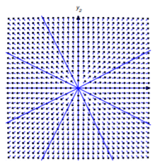
We leave it to you (Exercise 10.4.35) to classify the trajectories of Equation \ref{eq:10.4.18} if zero is an eigenvalue of \(A\). We’ll confine our attention here to the case where both eigenvalues are nonzero. In this case the simplest situation is where \(\lambda_1=\lambda_2\ne0\), so Equation \ref{eq:10.4.19} becomes
\[{\bf y}=(c_1{\bf x}_1+c_2{\bf x}_2)e^{\lambda_1 t}.\nonumber\]
Since \({\bf x}_1\) and \({\bf x}_2\) are linearly independent, an arbitrary vector \({\bf x}\) can be written as \({\bf x}=c_1{\bf x}_1+c_2{\bf x}_2\). Therefore the general solution of Equation \ref{eq:10.4.18} can be written as \({\bf y}={\bf x}e^{\lambda_1 t}\) where \({\bf x}\) is an arbitrary \(2\)-vector, and the trajectories of nontrivial solutions of Equation \ref{eq:10.4.18} are half-lines through (but not including) the origin. The direction of motion is away from the origin if \(\lambda_1>0\) (Figure 10.4.1 ), toward it if \(\lambda_1<0\) (Figure 10.4.2 ). (In these and the next figures an arrow through a point indicates the direction of motion along the trajectory through the point.)
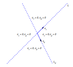
Now suppose \(\lambda_2>\lambda_1\), and let \(L_1\) and \(L_2\) denote lines through the origin parallel to \({\bf x}_1\) and \({\bf x}_2\), respectively. By a half-line of \(L_1\) (or \(L_2\)), we mean either of the rays obtained by removing the origin from \(L_1\) (or \(L_2\)).
Letting \(c_2=0\) in Equation \ref{eq:10.4.19} yields \({\bf y}=c_1{\bf x}_1e^{\lambda_1 t}\). If \(c_1\ne0\), the trajectory defined by this solution is a half-line of \(L_1\). The direction of motion is away from the origin if \(\lambda_1>0\), toward the origin if \(\lambda_1<0\). Similarly, the trajectory of \({\bf y}=c_2{\bf x}_2e^{\lambda_2 t}\) with \(c_2\ne0\) is a half-line of \(L_2\).
Henceforth, we assume that \(c_1\) and \(c_2\) in Equation \ref{eq:10.4.19} are both nonzero. In this case, the trajectory of Equation \ref{eq:10.4.19} can’t intersect \(L_1\) or \(L_2\), since every point on these lines is on the trajectory of a solution for which either \(c_1=0\) or \(c_2=0\). (Remember: distinct trajectories can’t intersect!). Therefore the trajectory of Equation \ref{eq:10.4.19} must lie entirely in one of the four open sectors bounded by \(L_1\) and \(L_2\), but do not any point on \(L_1\) or \(L_2\). Since the initial point \((y_1(0),y_2(0))\) defined by
\[{\bf y}(0)=c_1{\bf x}_1+c_2{\bf x}_2\nonumber\]
is on the trajectory, we can determine which sector contains the trajectory from the signs of \(c_1\) and \(c_2\), as shown in Figure 10.4.3 .
The direction of \({\bf y}(t)\) in Equation \ref{eq:10.4.19} is the same as that of
\[\label{eq:10.4.20} e^{-\lambda_2 t}{\bf y}(t)= c_1{\bf x}_1e^{-(\lambda_2-\lambda_1)t}+c_2{\bf x}_2\]
and of
\[\label{eq:10.4.21} e^{-\lambda_1 t}{\bf y}(t)=c_1{\bf x}_1+c_2{\bf x}_2e^{(\lambda_2-\lambda_1)t}.\]
Since the right side of Equation \ref{eq:10.4.20} approaches \(c_2{\bf x}_2\) as \(t\to\infty\), the trajectory is asymptotically parallel to \(L_2\) as \(t\to\infty\). Since the right side of Equation \ref{eq:10.4.21} approaches \(c_1{\bf x}_1\) as \(t\to-\infty\), the trajectory is asymptotically parallel to \(L_1\) as \(t\to-\infty\).
The shape and direction of traversal of the trajectory of Equation \ref{eq:10.4.19} depend upon whether \(\lambda_1\) and \(\lambda_2\) are both positive, both negative, or of opposite signs. We’ll now analyze these three cases.
Henceforth \(\|{\bf u}\|\) denote the length of the vector \({\bf u}\).
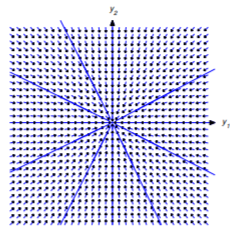
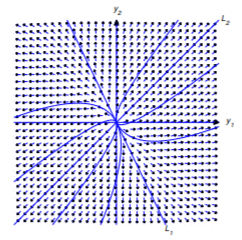
Case 1: \(\lambda _{2}>\lambda _{1}>0\)
Figure 10.4.4 shows some typical trajectories. In this case, \(\lim_{t\to-\infty}\|{\bf y}(t)\|=0\), so the trajectory is not only asymptotically parallel to \(L_1\) as \(t\to-\infty\), but is actually asymptotically tangent to \(L_1\) at the origin. On the other hand, \(\lim_{t\to\infty}\|{\bf y}(t)\|=\infty\) and
\[\lim_{t\to\infty}\left\|{\bf y}(t)-c_2{\bf x}_2e^{\lambda_2 t}\right\|=\lim_{t\to\infty}\|c_1{\bf x_1}e^{\lambda_1t}\|=\infty,\nonumber\]
so, although the trajectory is asymptotically parallel to \(L_2\) as \(t\to\infty\), it is not asymptotically tangent to \(L_2\). The direction of motion along each trajectory is away from the origin.
Case 2: \(0>\lambda _{2}>\lambda _{1}\)
Figure 10.4.5 shows some typical trajectories. In this case, \(\lim_{t\to\infty}\|{\bf y}(t)\|=0\), so the trajectory is asymptotically tangent to \(L_2\) at the origin as \(t\to\infty\). On the other hand, \(\lim_{t\to-\infty}\|{\bf y}(t)\|=\infty\) and
\[\lim_{t\to-\infty}\left\|{\bf y}(t)-c_1{\bf x}_1e^{\lambda_1 t}\right\|=\lim_{t\to-\infty}\|c_2{\bf x}_2e^{\lambda_2t}\|=\infty,\nonumber\]
so, although the trajectory is asymptotically parallel to \(L_1\) as \(t\to-\infty\), it is not asymptotically tangent to it. The direction of motion along each trajectory is toward the origin.
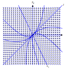
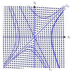
Case 3: \(\lambda _{2}>0>\lambda _{1}\)
Figure 10.4.6 shows some typical trajectories. In this case,
\[\lim_{t\to\infty}\|{\bf y}(t)\|=\infty \quad \text{and} \quad \lim_{t\to\infty}\left\|{\bf y}(t)-c_2{\bf x}_2e^{\lambda_2 t}\right\|=\lim_{t\to\infty}\|c_1{\bf x}_1e^{\lambda_1t}\|=0,\nonumber\]
so the trajectory is asymptotically tangent to \(L_2\) as \(t\to\infty\). Similarly,
\[\lim_{t\to-\infty}\|{\bf y}(t)\|=\infty \quad \text{and} \quad \lim_{t\to-\infty}\left\|{\bf y}(t)-c_1{\bf x}_1e^{\lambda_1 t}\right\|=\lim_{t\to-\infty}\|c_2{\bf x}_2e^{\lambda_2t}\|=0,\nonumber\]
so the trajectory is asymptotically tangent to \(L_1\) as \(t\to-\infty\). The direction of motion is toward the origin on \(L_1\) and away from the origin on \(L_2\). The direction of motion along any other trajectory is away from \(L_1\), toward \(L_2\).