2.2: Linear Second Order Constant Coefficient Homogeneous Equations

If \(a,b\), and \(c\) are real constants and \(a\ne0\), then

\begin{eqnarray*}
ay''+by'+cy=F(x)
\end{eqnarray*}

is said to be a \( \textcolor{blue}{\mbox{constant coefficient equation}} \) In this section we consider the homogeneous constant coefficient equation

\begin{equation}\label{eq:2.2.1}
ay''+by'+cy=0.
\end{equation}

As we'll see, all solutions of \eqref{eq:2.2.1} are defined on \((-\infty,\infty)\). This being the case, we'll omit references to the interval on which solutions are defined, or on which a given set of solutions is a fundamental set, etc., since the interval will always be \((-\infty,\infty)\).

The key to solving \eqref{eq:2.2.1} is that if \(y=e^{rx}\) where \(r\) is a constant then the left side of \eqref{eq:2.2.1} is a multiple of \(e^{rx}\); thus, if \(y=e^{rx}\) then \(y'=re^{rx}\) and \(y''=r^2e^{rx}\), so

\begin{equation}\label{eq:2.2.2}
ay''+by'+cy=ar^2e^{rx}+bre^{rx}+ce^{rx}=(ar^2+br+c)e^{rx}.
\end{equation}

The quadratic polynomial

\begin{eqnarray*}
p(r)=ar^2+br+c
\end{eqnarray*}

is the \( \textcolor{blue}{\mbox{characteristic polynomial}} \) of \eqref{eq:2.2.1}, and \(p(r)=0\) is the \( \textcolor{blue}{\mbox{characteristic equation}} \). From \eqref{eq:2.2.2} we can see that \(y=e^{rx}\) is a solution of \eqref{eq:2.2.1} if and only if \(p(r)=0\).

The roots of the characteristic equation are given by the quadratic formula

\begin{equation}\label{eq:2.2.3}
r={-b\pm\sqrt{b^2-4ac}\over2a}.
\end{equation}

We consider three cases:

Case 1. \(b^2-4ac>0\), so the characteristic equation has two distinct real roots.

Case 2. \(b^2-4ac=0\), so the characteristic equation has a repeated real root.

Case 3. \(b^2-4ac<0\), so the characteristic equation has complex roots.

In each case we'll start with an example.

Case 1: Distinct Real Roots

Example \(\PageIndex{1}\)

(a) Find the general solution of

\begin{equation}\label{eq:2.2.4}
y''+6y'+5y=0.
\end{equation}

(b) Solve the initial value problem

\begin{equation}\label{eq:2.2.5}
y''+6y'+5y=0, \quad y(0)=3,\; y'(0)=-1.
\end{equation}

Answer

(a) The characteristic polynomial of \eqref{eq:2.2.4} is

\begin{eqnarray*}
p(r)=r^2+6r+5=(r+1)(r+5).
\end{eqnarray*}

Since \(p(-1)=p(-5)=0\), \(y_1=e^{-x}\) and \(y_2=e^{-5x}\) are solutions of \eqref{eq:2.2.4}. Since \(y_2/y_1=e^{-4x}\) is nonconstant, Theorem \((2.1.6)\) implies that the general solution of \eqref{eq:2.2.4} is

\begin{equation}\label{eq:2.2.6}
y=c_1e^{-x}+c_2e^{-5x}.
\end{equation}

(b) We must determine \(c_1\) and \(c_2\) in \eqref{eq:2.2.6} so that \(y\) satisfies the initial conditions in \eqref{eq:2.2.5}. Differentiating \eqref{eq:2.2.6} yields

\begin{equation}\label{eq:2.2.7}
y'=-c_1e^{-x}-5c_2e^{-5x}.
\end{equation}

Imposing the initial conditions \(y(0)=3,\, y'(0)=-1\) in \eqref{eq:2.2.6} and \eqref{eq:2.2.7} yields

\begin{eqnarray*}
\begin{array}{rcr}
\phantom{-}c_1+\phantom{5}c_2 & = & 3\phantom{.}\\
-c_1-5c_2 & = & -1.
\end{array}
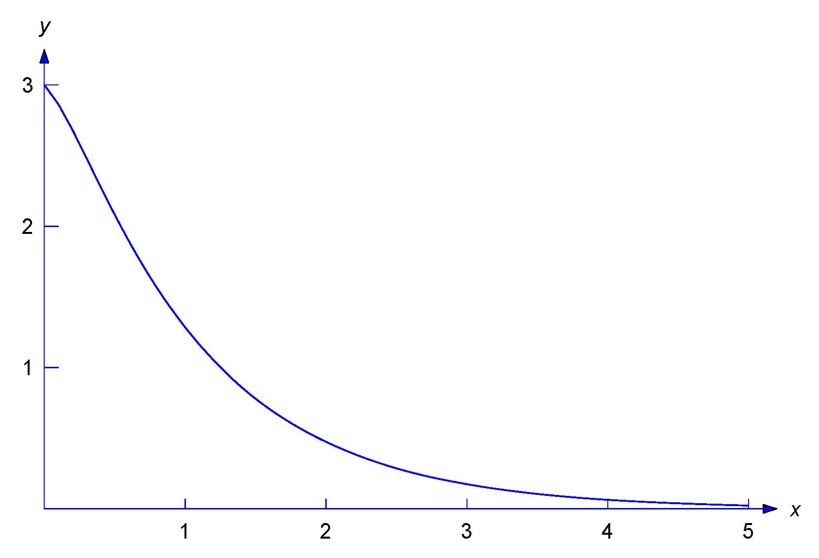
\end{eqnarray*}

The solution of this system is \(c_1=7/2,c_2=-1/2\). Therefore the solution of \eqref{eq:2.2.5} is

\begin{eqnarray*}
y={7\over2}e^{-x}-{1\over2}e^{-5x}.
\end{eqnarray*}

Figure \(2.2.1\) is a graph of this solution.

Figure: \(2.2.1\)

\(y = \displaystyle\frac{7}{2} e^{-x} - \displaystyle\frac{1}{2} e^{-5x} \)

If the characteristic equation has arbitrary distinct real roots \(r_1\) and \(r_2\), then \(y_1=e^{r_1x}\) and \(y_2=e^{r_2x}\) are solutions of \(ay''+by'+cy=0\). Since \(y_2/y_1=e^{(r_2-r_1)x}\) is nonconstant, Theorem \((2.1.6)\) implies that \(\{y_1,y_2\}\) is a fundamental set of solutions of \(ay''+by'+cy=0\).

Case 2: A Repeated Real Root

Example \(\PageIndex{2}\)

(a) Find the general solution of

\begin{equation}\label{eq:2.2.8}
y''+6y'+9y=0.
\end{equation}

(b) Solve the initial value problem

\begin{equation}\label{eq:2.2.9}
y''+6y'+9y=0, \quad y(0)=3,\; y'(0)=-1.
\end{equation}

Answer

(a) The characteristic polynomial of \eqref{eq:2.2.8} is

\begin{eqnarray*}
p(r)=r^2+6r+9=(r+3)^2,
\end{eqnarray*}

so the characteristic equation has the repeated real root \(r_1=-3\). Therefore \(y_1=e^{-3x}\) is a solution of \eqref{eq:2.2.8}. Since the characteristic equation has no other roots, \eqref{eq:2.2.8} has no other solutions of the form \(e^{rx}\). We look for solutions of the form \(y=uy_1=ue^{-3x}\), where \(u\) is a function that we'll now determine.

This should remind you of the method of variation of parameters used in Section 2.1 to solve the nonhomogeneous equation \(y'+p(x)y=f(x)\), given a solution \(y_1\) of the complementary equation \(y'+p(x)y=0\). It's also a special case of a method called \( \textcolor{blue}{\mbox{reduction of order}} \) that we'll study in Section 5.6. For other ways to obtain a second solution of \eqref{eq:2.2.8} that's not a multiple of \(e^{-3x}\), see Exercises \((2.1E.9)\), \((2.1E.12)\), and \((2.2E.33)\).

If \(y=ue^{-3x}\), then

\begin{eqnarray*}
y'=u'e^{-3x}-3ue^{-3x} \quad \mbox{and} \quad y''=u''e^{-3x}-6u'e^{-3x}+9ue^{-3x},
\end{eqnarray*}

so

\begin{eqnarray*}
y''+6y'+9y&=&e^{-3x}\left[(u''-6u'+9u)+6(u'-3u)+9u\right]\\
&=&e^{-3x}\left[u''-(6-6)u'+(9-18+9)u\right]=u''e^{-3x}.
\end{eqnarray*}

Therefore \(y=ue^{-3x}\) is a solution of \eqref{eq:2.2.8} if and only if \(u''=0\), which is equivalent to \(u=c_1+c_2x\), where \(c_1\) and \(c_2\) are constants. Therefore any function of the form

\begin{equation}\label{eq:2.2.10}
y=e^{-3x}(c_1+c_2x)
\end{equation}

is a solution of \eqref{eq:2.2.8}. Letting \(c_1=1\) and \(c_2=0\) yields the solution \(y_1=e^{-3x}\) that we already knew. Letting \(c_1=0\) and \(c_2=1\) yields the second solution \(y_2=xe^{-3x}\). Since \(y_2/y_1=x\) is nonconstant, Theorem \((2.1.6)\) implies that \(\{y_1,y_2\}\) is fundamental set of solutions of \eqref{eq:2.2.8}, and \eqref{eq:2.2.10} is the general solution.

(b) Differentiating \eqref{eq:2.2.10} yields

\begin{equation}\label{eq:2.2.11}
y'=-3e^{-3x}(c_1+c_2x)+c_2e^{-3x}.
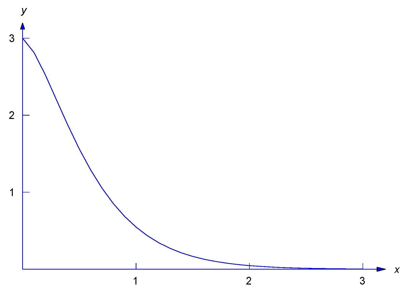
\end{equation}

Imposing the initial conditions \(y(0)=3,\, y'(0)=-1\) in \eqref{eq:2.2.10} and \eqref{eq:2.2.11} yields \(c_1=3\) and \(-3c_1+c_2=-1\), so \(c_2=8\). Therefore the solution of \eqref{eq:2.2.9} is

\begin{eqnarray*}
y=e^{-3x}(3+8x).
\end{eqnarray*}

Figure \(2.2.2\) is a graph of this solution.

Figure: \(2.2.2\)

\(y=e^{-3x}(3+8x)\)

If the characteristic equation of \(ay''+by'+cy=0\) has an arbitrary repeated root \(r_1\), the characteristic polynomial must be

\begin{eqnarray*}
p(r)=a(r-r_1)^2=a(r^2-2r_1r+r_1^2).
\end{eqnarray*}

Therefore

\begin{eqnarray*}
ar^2+br+c=ar^2-(2ar_1)r+ar_1^2,
\end{eqnarray*}

which implies that \(b=-2ar_1\) and \(c=ar_1^2\). Therefore \(ay''+by'+cy=0\) can be written as \(a(y''-2r_1y'+r_1^2y)=0\). Since \(a\ne0\) this equation has the same solutions as

\begin{equation}\label{eq:2.2.12}
y''-2r_1y'+r_1^2y=0.
\end{equation}

Since \(p(r_1)=0\), \(y_1=e^{r_1x}\) is a solution of \(ay''+by'+cy=0\), and therefore of \eqref{eq:2.2.12}. Proceeding as in Example \((2.2.2)\), we look for other solutions of \eqref{eq:2.2.12} of the form \(y=ue^{r_1x}\); then

\begin{eqnarray*}
y'=u'e^{r_1x}+rue^{r_1x} \quad \mbox{and} \quad y''=u''e^{r_1x}+2r_1u'e^{r_1x}+r_1^2ue^{r_1x},
\end{eqnarray*}

so

\begin{eqnarray*}
y''-2r_1y'+r_1^2y&=&e^{rx}\left[(u''+2r_1u'+r_1^2u) - 2r_1(u'+r_1u)+r_1^2u\right]\\
&=&e^{r_1x}\left[u''+(2r_1-2r_1)u'+(r_1^2-2r_1^2+r_1^2)u\right]=u''e^{r_1x}.
\end{eqnarray*}

Therefore \(y=ue^{r_1x}\) is a solution of \eqref{eq:2.2.12} if and only if \(u''=0\), which is equivalent to \(u=c_1+c_2x\), where \(c_1\) and \(c_2\) are constants. Hence, any function of the form

\begin{equation}\label{eq:2.2.13}
y=e^{r_1x}(c_1+c_2x)
\end{equation}

is a solution of \eqref{eq:2.2.12}. Letting \(c_1=1\) and \(c_2=0\) here yields the solution \(y_1=e^{r_1x}\) that we already knew. Letting \(c_1=0\) and \(c_2=1\) yields the second solution \(y_2=xe^{r_1x}\). Since \(y_2/y_1=x\) is nonconstant, Theorem \((2.1.6)\) implies that \(\{y_1,y_2\}\) is a fundamental set of solutions of \eqref{eq:2.2.12}, and \eqref{eq:2.2.13} is the general solution.

Case 3: Complex Conjugate Roots

Example \(\PageIndex{3}\)

(a) Find the general solution of

\begin{equation}\label{eq:2.2.14}
y''+4y'+13y=0.
\end{equation}

(b) Solve the initial value problem

\begin{equation}\label{eq:2.2.15}
y''+4y'+13y=0, \quad y(0)=2,\; y'(0)=-3.
\end{equation}

Answer

(a) The characteristic polynomial of \eqref{eq:2.2.14} is

\begin{eqnarray*}
p(r)=r^2+4r+13=r^2+4r+4+9=(r+2)^2+9.
\end{eqnarray*}

The roots of the characteristic equation are \(r_1=-2+3i\) and \(r_2=-2-3i\). By analogy with Case 1, it's reasonable to expect that \(e^{(-2+3i)x}\) and \(e^{(-2-3i)x}\) are solutions of \eqref{eq:2.2.14}. This is true (see Exercise \((2.2E.34)\)); however, there are difficulties here, since you are probably not familiar with exponential functions with complex arguments, and even if you are, it's inconvenient to work with them, since they are complex--valued. We'll take a simpler approach, which we motivate as follows: the exponential notation suggests that

\begin{eqnarray*}
e^{(-2+3i)x}=e^{-2x}e^{3ix} \quad \mbox{and} \quad e^{(-2-3i)x}=e^{-2x}e^{-3ix},
\end{eqnarray*}

so even though we haven't defined \(e^{3ix}\) and \(e^{-3ix}\), it's reasonable to expect that every linear combination of \(e^{(-2+3i)x}\) and \(e^{(-2-3i)x}\) can be written as \(y=ue^{-2x}\), where \(u\) depends upon \(x\). To determine \(u\), we note that if \(y=ue^{-2x}\) then

\begin{eqnarray*}
y'=u'e^{-2x}-2ue^{-2x} \quad \mbox{and} \quad y''=u''e^{-2x}-4u'e^{-2x}+4ue^{-2x},
\end{eqnarray*}

so

\begin{eqnarray*}
y''+4y'+13y&=&e^{-2x}\left[(u''-4u'+4u)+4(u'-2u)+13u\right]\\
&=&e^{-2x}\left[u''-(4-4)u'+(4-8+13)u\right]=e^{-2x}(u''+9u).
\end{eqnarray*}

Therefore \(y=ue^{-2x}\) is a solution of \eqref{eq:2.2.14} if and only if

\begin{eqnarray*}
u''+9u=0.
\end{eqnarray*}

From Example \((2.1.2)\), the general solution of this equation is

\begin{eqnarray*}
u=c_1\cos 3x +c_2\sin 3x.
\end{eqnarray*}

Therefore any function of the form

\begin{equation}\label{eq:2.2.16}
y=e^{-2x}(c_1\cos 3x+c_2\sin 3x)
\end{equation}

is a solution of \eqref{eq:2.2.14}. Letting \(c_1=1\) and \(c_2=0\) yields the solution \(y_1=e^{-2x}\cos3x\). Letting \(c_1=0\) and \(c_2=1\) yields the second solution \(y_2=e^{-2x}\sin3x\). Since \(y_2/y_1=\tan3x\) is nonconstant, Theorem \((2.1.6)\) implies that \(\{y_1,y_2\}\) is a fundamental set of solutions of \eqref{eq:2.2.14}, and \eqref{eq:2.2.16} is the general solution.

(b) Imposing the condition \(y(0)=2\) in \eqref{eq:2.2.16} shows that \(c_1=2\). Differentiating \eqref{eq:2.2.16} yields

\begin{eqnarray*}
y'=-2e^{-2x}(c_1\cos 3x+c_2\sin 3x) +3e^{-2x}(-c_1\sin 3x +c_2\cos 3x),
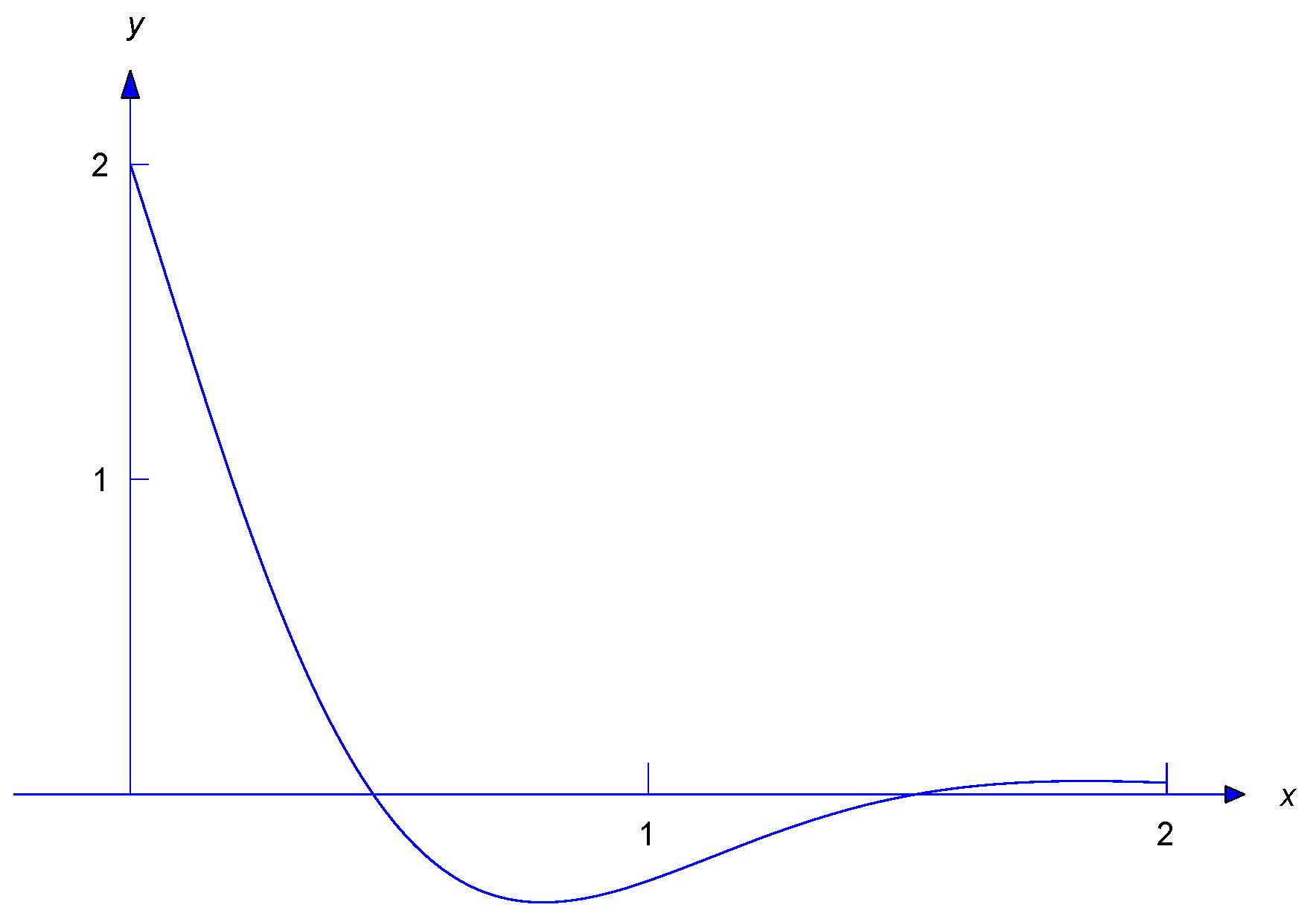
\end{eqnarray*}

and imposing the initial condition \(y'(0)=-3\) here yields \(-3=-2c_1+3c_2=-4+3c_2\), so \(c_2=1/3\). Therefore the solution of \eqref{eq:2.2.15} is

\begin{eqnarray*}
y=e^{-2x}(2\cos 3x+ {1\over3}\sin 3x).
\end{eqnarray*}

Figure \(2.2.3\) Is a graph of this function.

Figure: \(2.2.3\)

\(\displaystyle{y=e^{-2x}(2\cos 3x+ {1\over3}\sin 3x)}\)

Now suppose the characteristic equation of \(ay''+by'+cy=0\) has arbitrary complex roots; thus, \(b^2-4ac<0\) and, from \eqref{eq:2.2.3}, the roots are

\begin{eqnarray*}
r_1 = {-b+i\sqrt{4ac-b^2}\over 2a},\quad r_2 = {-b-i\sqrt{4ac-b^2}\over 2a},
\end{eqnarray*}

which we rewrite as

\begin{equation}\label{eq:2.2.17}
r_1=\lambda+i \omega,\quad r_2 = \lambda - i \omega,
\end{equation}

with

\begin{eqnarray*}
\lambda = -{b\over 2a},\quad \omega = {\sqrt{4ac-b^2}\over 2a}.
\end{eqnarray*}

Don't memorize these formulas. Just remember that \(r_1\) and \(r_2\) are of the form \eqref{eq:2.2.17}, where \(\lambda\) is an arbitrary real number and \(\omega\) is positive; \(\lambda\) and \(\omega\) are the \( \textcolor{blue}{\mbox{real}} \) and \( \textcolor{blue}{\mbox{imaginary parts}} \), respectively, of \(r_1\). Similarly, \(\lambda\) and \(-\omega\) are the real and imaginary parts of \(r_2\). We say that \(r_1\) and \(r_2\) are \( \textcolor{blue}{\mbox{complex conjugates}} \), which means that they have the same real part and their imaginary parts have the same absolute values, but opposite signs.

As in Example \((2.2.3)\), it's reasonable to to expect that the solutions of \(ay''+by'+cy=0\) are linear combinations of \(e^{(\lambda+i\omega)x}\) and \(e^{(\lambda-i\omega)x}\). Again, the exponential notation suggests that

\begin{eqnarray*}
e^{(\lambda+i\omega)x}=e^{\lambda x}e^{i\omega x} \quad \mbox{and} \quad e^{(\lambda-i\omega)x}=e^{\lambda x}e^{-i\omega x},
\end{eqnarray*}

so even though we haven't defined \(e^{i\omega x}\) and \(e^{-i\omega x}\), it's reasonable to expect that every linear combination of \(e^{(\lambda+i\omega)x}\) and \(e^{(\lambda-i\omega)x}\) can be written as \(y=ue^{\lambda x}\), where \(u\) depends upon \(x\). To determine \(u\) we first observe that since \(r_1=\lambda+i\omega\) and \(r_2=\lambda-i\omega\) are the roots of the characteristic equation, \(p\) must be of the form

\begin{eqnarray*}
\begin{array}{ccl}
p(r)&=&a(r-r_1)(r-r_2)\\
&=&a(r-\lambda-i\omega)(r-\lambda+i\omega)\\
&=& a \left[(r-\lambda)^2+\omega^2\right]\\
&=&a(r^2-2\lambda r +\lambda^2+\omega^2).
\end{array}
\end{eqnarray*}

Therefore \(ay''+by'+cy=0\) can be written as

\begin{eqnarray*}
a\left[y''-2\lambda y'+(\lambda^2+\omega^2)y\right]=0.
\end{eqnarray*}

Since \(a\ne0\) this equation has the same solutions as

\begin{equation}\label{eq:2.2.18}
y''-2\lambda y'+(\lambda^2+\omega^2)y=0.
\end{equation}

To determine \(u\) we note that if \(y=ue^{\lambda x}\) then

\begin{eqnarray*}
y'=u'e^{\lambda x}+\lambda ue^{\lambda x} \quad \mbox{and} \quad y''=u''e^{\lambda x}+2\lambda u'e^{\lambda x}+\lambda^2ue^{\lambda x}.
\end{eqnarray*}

Substituting these expressions into \eqref{eq:2.2.18} and dropping the common factor \(e^{\lambda x}\) yields

\begin{eqnarray*}
(u''+2\lambda u'+\lambda^2 u)-2\lambda(u'+\lambda u) + (\lambda^2+\omega^2)u=0,
\end{eqnarray*}

which simplifies to

\begin{eqnarray*}
u''+\omega^2 u=0.
\end{eqnarray*}

From Example \((2.1.2)\), the general solution of this equation is

\begin{eqnarray*}
u=c_1\cos\omega x +c_2\sin\omega x.
\end{eqnarray*}

Therefore any function of the form

\begin{equation}\label{eq:2.2.19}
y=e^{\lambda x}(c_1\cos\omega x+c_2\sin\omega x)
\end{equation}

is a solution of \eqref{eq:2.2.18}. Letting \(c_1=1\) and \(c_2=0\) here yields the solution \(y_1=e^{\lambda x}\cos\omega x\). Letting \(c_1=0\) and \)c_2=1\) yields a second solution \(y_2=e^{\lambda x}\sin\omega x\). Since \(y_2/y_1=\tan\omega x\) is nonconstant, so Theorem \((2.1.6)\) implies that \(\{y_1,y_2\}\) is a fundamental set of solutions of \eqref{eq:2.2.18}, and \eqref{eq:2.2.19} is the general solution.

Summary

The next theorem summarizes the results of this section.

Theorem \(\PageIndex{1}\)

Let \(p(r)=ar^2+br+c\) be the characteristic polynomial of

\begin{equation}\label{eq:2.2.20}
ay''+by'+cy=0.
\end{equation}

Then\(:\)

(a) If \(p(r)=0\) has distinct real roots \(r_1\) and \(r_2,\) then the general solution of \eqref{eq:2.2.20} is

\begin{eqnarray*}
y=c_1e^{r_1x}+c_2e^{r_2x}.
\end{eqnarray*}

(b) If \(p(r)=0\) has a repeated root \(r_1,\) then the general solution of \eqref{eq:2.2.20} is

\begin{eqnarray*}
y=e^{r_1x}(c_1+c_2x).
\end{eqnarray*}

(c) If \(p(r)=0\) has complex conjugate roots \(r_1=\lambda+i\omega\) and \(r_2=\lambda-i\omega\) \((\)where \(\omega>0),\) then the general solution of \eqref{eq:2.2.20} is

\begin{eqnarray*}
y=e^{\lambda x}(c_1\cos\omega x+c_2\sin\omega x).
\end{eqnarray*}

Proof

Add proof here and it will automatically be hidden if you have a "AutoNum" template active on the page.