2.11E: Exercises for Lagrange Multipliers
- Last updated
- Save as PDF
- Page ID
- 54044
In exercises 1-15, use the method of Lagrange multipliers to find the maximum and minimum values of the function subject to the given constraint.
1) Objective function: \(f(x, y) = 4xy\) Constraint: \(\dfrac{x^2}{9} + \dfrac{y^2}{16} = 1\)
- Answer
- Subject to the given constraint, the function \(f\) has a relative minimum of \(-24\) at both \( \left(-\frac{3\sqrt{2}}{2}, 2\sqrt{2}\right) \) and \( \left(\frac{3\sqrt{2}}{2}, -2\sqrt{2}\right) \) and a relative maximum of \(24\) at both \( \left(\frac{3\sqrt{2}}{2}, 2\sqrt{2}\right) \) and \( \left(-\frac{3\sqrt{2}}{2}, -2\sqrt{2}\right) \)
2) Objective function: \(f(x, y) = x^2y\) Constraint: \(x^2 + 2y^2 = 6\)
3) Objective function: \(f(x,y)=x^2 +y^2 +2x−2y+1\) Constraint: \( g(x,y)= x^2 +y^2 =2 \)
- Answer
- Subject to the given constraint, \(f\) has a relative minimum of \(-1\) at \( (-1, 1) \) and a relative maximum of \(7\) at \( (1,-1) \).
4) Objective function: \(f(x, y) = xy\) Constraint: \(4x^2 + 8y^2 = 16\)
5) Objective function: \(f(x, y) = x^2 + y^2\) Constraint: \(xy = 1\)
- Answer
- \(f\) has a relative minimum of \(2\) at both \( (-1, -1) \) and \( (1,1) \), subject to the given constraint.
6) Objective function: \(f(x, y) = x^2 - y^2\) Constraint: \(x−2y+6=0\)
7) Objective function: \(f(x, y) = x^2 + y^2\) Constraint: \(x+2y−5=0\)
- Answer
- Subject to the given constraint, \(f\) has a relative minimum of \( f(1,2)=5\) at the point \( (1, 2) \).
8) Objective function: \(f(x, y) = x^2 + y^2\) Constraint: \((x−1)^2+4y^2=4\)
9) Objective function: \(f(x, y) = 4x^3 + y^2\) Constraint: \(2x^2 + y^2 = 1\)
- Answer
- Subject to the given constraint, the function \(f\) has a relative minimum of \(-\sqrt{2}\) at \( \left(-\frac{\sqrt{2}}{2}, 0\right) \),
a relative minimum of \(\frac{25}{27}\) at both points \( \left(\frac{1}{3}, -\frac{\sqrt{7}}{3}\right) \) and \( \left(\frac{1}{3}, \frac{\sqrt{7}}{3}\right) \),
a relative maximum of \(\sqrt{2}\) at \( \left(\frac{\sqrt{2}}{2}, 0\right) \), and a relative maximum of \(1\) at both points \( (0,1) \) and \( (0,-1) \).
- Solution:
- Let \(g(x,y) = 2x^2 + y^2\) be the constraint function. Then:
\(\vecs\nabla f(x,y) = 12x^2 \,\hat{\mathbf i} + 2y \,\hat{\mathbf j}\) and \(\vecs\nabla g(x,y) = 4x \,\hat{\mathbf i} + 2y \,\hat{\mathbf j}\)
Using the Lagrange Multiplier equation, \[\vecs\nabla f(x, y) = \lambda\vecs\nabla g(x, y),\nonumber \]
we have: \[12x^2 \,\hat{\mathbf i} + 2y \,\hat{\mathbf j} = 4x\lambda \, \hat{\mathbf i} + 2y\lambda \,\hat{\mathbf j}\nonumber \]
giving us the system of equations: \[12x^2 = 4x\lambda, \quad 2y = 2y\lambda, \quad \text{and the constraint}\quad 2x^2 + y^2 = 1\nonumber \]
Rewriting the first two equations as zero-products (by moving to one-side and factoring), we get:
\[\begin{align*} 4x(3x - \lambda) &= 0 & \text{and} && 2y(1 - \lambda) &= 0 \\ x = 0 \quad \text{or}\quad \lambda &= 3x & & &y = 0 \quad \text{or}\quad \lambda &= 1 \end{align*}\]
Now we consider the combinations of these solutions to the above two equations and plug each of these into the constraint equation to solve for the corresponding Lagrange points.
The combination \(x = 0\) and \(y = 0\) produces a contradiction when placed in the constraint equation, since this point is not on the ellipse.
Taking the combination \(x = 0\) and \(\lambda = 1\), we put \(0\) in for \(x\) in the constraint and solve for \(y\), obtaining: \( y = \pm 1\). This gives us two Lagrange points: \( (0, 1) \) and \( (0, -1)\).
Taking the combination \(\lambda = 3x\) and \(y = 0\), we put \(0\) in for \(y\) in the constraint and solve for \(x\), obtaining: \( x = \pm \frac{\sqrt{2}}{2}\). This gives us two Lagrange points: \( \left(-\frac{\sqrt{2}}{2}, 0\right) \) and \( \left(\frac{\sqrt{2}}{2}, 0\right) \).
Taking the combination \(\lambda = 3x\) and \(\lambda = 1\), we substitute \(1\) into the first equation for \(\lambda\), giving us \( 1 = 3x\) so \(x = \frac{1}{3}\). Plugging this value in for \(x\) in the constraint equation and solving for \(y\), we obtain \(y = \pm \frac{\sqrt{7}}{3}\) which gives us the two Lagrange points: \( \left(\frac{1}{3}, -\frac{\sqrt{7}}{3}\right) \) and \( \left(\frac{1}{3}, \frac{\sqrt{7}}{3}\right) \).
Evaluating the function \(f\) at these Lagrange points, we find: \[\begin{align*} f(0, -1) &= 1 & f(0, 1) &= 1 \\ f\left(-\tfrac{\sqrt{2}}{2}, 0\right) &= \frac{-4(\sqrt{2})^3}{8} = -\sqrt{2} & f\left(\tfrac{\sqrt{2}}{2}, 0\right) &= \frac{4(\sqrt{2})^3}{8} = \sqrt{2} \\ f\left(\tfrac{1}{3}, -\tfrac{\sqrt{7}}{3}\right) &= \tfrac{25}{27} & f\left(\tfrac{1}{3}, \tfrac{\sqrt{7}}{3}\right) &= \tfrac{25}{27} \end{align*}\]
Comparing these values with where the corresponding Lagrange points lie on the constraint curve, we conclude the results stated in the answer above.
10) Objective function: \(f(x,y)=2x^2 +y^2\) Constraint: \( g(x,y)= x^2 +y^2 =1 \)
11) Objective function: \(f(x,y,z)=x+3y−z\) Constraint: \( x^2+y^2+z^2=4 \)
- Answer
- Subject to the given constraint,\(f\) has a relative minimum of \(-2\sqrt{11}\) at the point \( \left(-\frac{2\sqrt{11}}{11}, \, -\frac{6\sqrt{11}}{11}, \, \frac{2\sqrt{11}}{11}\right) \) and a relative maximum of \(2\sqrt{11}\) at the point \( \left(\frac{2\sqrt{11}}{11}, \, \frac{6\sqrt{11}}{11}, \, -\frac{2\sqrt{11}}{11}\right).\)
12) Objective function: \(f(x, y, z) = x + y + z\) Constraint: \(\dfrac{1}{x}+\dfrac{1}{y}+\dfrac{1}{z}=1\)
13) Objective function: \(f(x, y, z) = xyz\) Constraint: \(x^2+2y^2+3z^2=6\)
- Answer
- Subject to the given constraint, \(f\) has a relative minimum of \(-\frac{2\sqrt{3}}{3}\) at \( \left( \sqrt{2},\, 1,\, -\frac{\sqrt{6}}{3} \right),\; \left( \sqrt{2},\, -1,\, \frac{\sqrt{6}}{3} \right),\; \left( -\sqrt{2},\, 1,\, \frac{\sqrt{6}}{3} \right),\) and \( \left( -\sqrt{2},\, -1,\, -\frac{\sqrt{6}}{3} \right) \) and a relative maximum of \(\frac{2\sqrt{3}}{3}\) at \( \left( \sqrt{2},\, 1,\, \frac{\sqrt{6}}{3} \right),\; \left( \sqrt{2},\, -1,\, -\frac{\sqrt{6}}{3} \right),\; \left( -\sqrt{2},\, -1,\, \frac{\sqrt{6}}{3} \right),\) and \( \left( -\sqrt{2},\, 1,\, -\frac{\sqrt{6}}{3} \right) \).
14) Objective function: \(f(x, y, z) = x^2 + y^2 + z^2\) Constraint: \(x^4+y^4+z^4=1\)
15) Objective function: \(f(x, y, z) = x^2 + y^2 + z^2\) Constraint: \(xyz=4\)
- Answer
- Subject to the given constraint, \(f\) has a relative minimum of \( 6\sqrt[3]{2}\) at the points \( \left(\sqrt[3]{4},\,\sqrt[3]{4},\,\sqrt[3]{4}\right),\) \( \left(\sqrt[3]{4},\,-\sqrt[3]{4},\,-\sqrt[3]{4}\right),\) \( \left(-\sqrt[3]{4},\,\sqrt[3]{4},\,-\sqrt[3]{4}\right),\) and \( \left(-\sqrt[3]{4},\,-\sqrt[3]{4},\,\sqrt[3]{4}\right).\)
To see a 3D visualization of this problem, see: CalcPlot3D for Problem 15.
In exercises 16-21, use the method of Lagrange multipliers to find the requested extremum of the given function subject to the given constraint.
16) Maximize \(f(x,y) = \sqrt{6 - x^2 - y^2}\) subject to the constraint, \( x+y−2=0\).
17) Maximize \(f(x,y) = x^2 - y^2\) subject to the constraints, \( g(x,y)=y−x^2=0, \quad x>0,\quad y>0\).
- Answer
- Subject to the given constraints, \(f\) has a relative maximum of \( f\left(\frac{\sqrt{2}}{2},\,\frac{1}{2}\right)=\frac{1}{4}\) at the point \( \left(\frac{\sqrt{2}}{2},\,\frac{1}{2}\right) \). If \(x > 0\) were not a constraint, there would have been two other Lagrange points with relative extrema of \(f\) subject to the other two constraints. These would have been \( (0, 0) \) and \( \left(-\frac{\sqrt{2}}{2},\,\frac{1}{2}\right) .\)
To verify that \(f\) really has a relative maximum at the point \( \left(\frac{\sqrt{2}}{2},\,\frac{1}{2}\right), \) we would need to check the value of \(f\) on either side of this point on the constraint curve, \(y−x^2=0.\)
If \( x = 0.5\) which is less than \(\frac{\sqrt{2}}{2}\), \(y\) would be \( y = (0.5)^2 = 0.25.\)
If \( x = 1\) which is greater than \(\frac{\sqrt{2}}{2}\), \(y\) would be \( y = (1)^2 = 1.\)
Then we compare the value of \(f\) at the Lagrange point, \(\left(\frac{\sqrt{2}}{2},\,\frac{1}{2}\right)\), with the values of \(f\) at these other points on the constraint.
We have \(f(0.5, 0.25) = (0.5)^2 - (0.25)^2 = 0.25 - 0.0625 = 0.1875 < \frac{1}{4}\) and \(f(1, 1) = (1)^2 - (1)^2 = 0 < \frac{1}{4}.\)
Therefore, we can conclude that \(f\) indeed has a relative maximum of \(\frac{1}{4}\) at the point \(\left(\frac{\sqrt{2}}{2},\,\frac{1}{2}\right).\)
18) Maximize \(U(x,y) = 8x^{4/5}y^{1/5}\) subject to the constraint, \( 4x+2y=12\).
19) Minimize \(f(x,y,z)=x^2+y^2+z^2\) subject to the constraint, \(x+y+z=1\).
- Answer
- Subject to the given constraint, \(f\) has a relative minimum of \( f\left(\frac{1}{3},\,\frac{1}{3},\,\frac{1}{3}\right)=\frac{1}{3}\) at the point \( \left(\frac{1}{3},\,\frac{1}{3},\,\frac{1}{3}\right) \).
20) Minimize \(f(x,y)=xy\) on the ellipse \(\dfrac{x^2}{a^2}+\dfrac{y^2}{b^2}=1\).
21) Maximize \(f(x,y,z)=2x+3y+5z\) on the sphere \(x^2+y^2+z^2=19\).
- Answer
- Subject to the given constraint, \(f\) has a relative maximum of \( 19\sqrt{2} \) at the point \( \left( \sqrt{2},\, \frac{3\sqrt{2}}{2},\, \frac{5\sqrt{2}}{2} \right) \).
Note that, subject to this constraint, \(f\) also has a relative minimum of \( -19\sqrt{2} \) at the point \( \left( -\sqrt{2},\, -\frac{3\sqrt{2}}{2},\, -\frac{5\sqrt{2}}{2} \right) \).
To see a 3D visualization of this problem, see: CalcPlot3D for Problem 21.
In exercises 22-23, use the method of Lagrange multipliers with two constraints.
22) Optimize \(f(x,y,z)=yz+xy\) subject to the constraints: \(xy=1, \quad y^2+z^2=1\).
- Answer
- maximum: \(\frac{3}{2}\), minimum: \(\frac{1}{2}\)
23) Minimize \(f(x,y,z)=x^2+y^2+z^2\) when \(x+y+z=9\) and \(x+2y+3z=20\).
- Answer
- minimum: \(f(2,3,4)=29\)
Use the method of Lagrange multipliers to solve the following applied problems.
24) A large container in the shape of a rectangular solid must have a volume of 480 m3. The bottom of the container costs $5/m2 to construct whereas the top and sides cost $3/m2 to construct. Use Lagrange multipliers to find the dimensions of the container of this size that has the minimum cost.
25) A rectangular box without a top (a topless box) is to be made from 12 ft2 of cardboard. Find the maximum volume of such a box.
- Answer
- The maximum volume is \(4\) ft3. The dimensions are \(1×2×2\) ft.
26) Find the minimum distance from the parabola \(y=x^2\) to point \((0,3)\).
27) Find the point on the line \(y=2x+3\) that is closest to point \((4,2)\).
- Answer
- \( (25,195) \)
29) Find the minimum distance from point \((0,1)\) to the parabola \(x^2=4y.\)
- Answer
- \(1.0\) unit
30) Find the minimum and maximum distances between the ellipse \(x^2+xy+2y^2=1\) and the origin.
31) Find the minimum distance from the plane \(x+y+z=1\) to point \((2,1,1)\).
- Answer
- \(\sqrt{3}\) units
32) Find the point on the plane \(4x+3y+z=2 \) that is closest to the point \((1,−1,1)\).
33) Find the point on the surface \(x^2−2xy+y^2−x+y=0\) closest to the point \((1,2,−3).\)
- Answer
- \( \left(1,\,\frac{1}{2},\,−3\right) \)
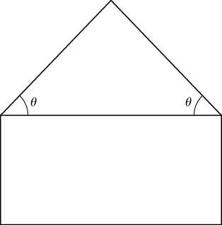
34) A pentagon is formed by placing an isosceles triangle on a rectangle, as shown in the diagram. If the perimeter of the pentagon is 10 in., find the lengths of the sides of the pentagon that will maximize the area of the pentagon.
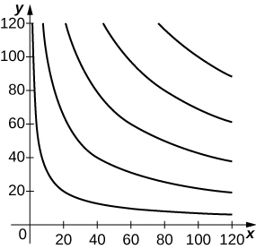
35) [T] By investing \(x\) units of labor and \(y\) units of capital, a watch manufacturer can produce \(P(x,y)=50x^{0.4}y^{0.6}\) watches. Find the maximum number of watches that can be produced on a budget of $20,000 if labor costs $100/unit and capital costs $200/unit. Use a grapher like CalcPlot3D to sketch a contour plot of the function.
- Answer
-
Roughly 3365 watches at the critical point (\(80,60).\)
36) A rectangular solid is contained within a tetrahedron with vertices at \((1,0,0),\,(0,1,0),\,(0,0,1)\), and the origin. The base of the box has dimensions \(x\) and \(y\), and the height of the box is \(z\). If the sum of \(x\), \(y\), and \(z\) is \(1\), find the dimensions that maximizes the volume of the rectangular solid.
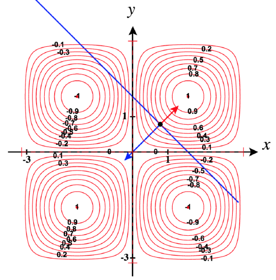
37) Find the maximum value of \(f(x,y)=\sin x\sin y,\) where \(x\) and \(y\) denote the acute angles of a right triangle. Draw the surface plot and contour plot of the function using a CAS.
- Answer
-
Subject to this constraint, \(f\) has a relative maximum of \(\frac{1}{2}\) when \(x = \frac{\pi}{4}\) and \(y = \frac{\pi}{4}\).
Surface plot and contour plot for\(f\):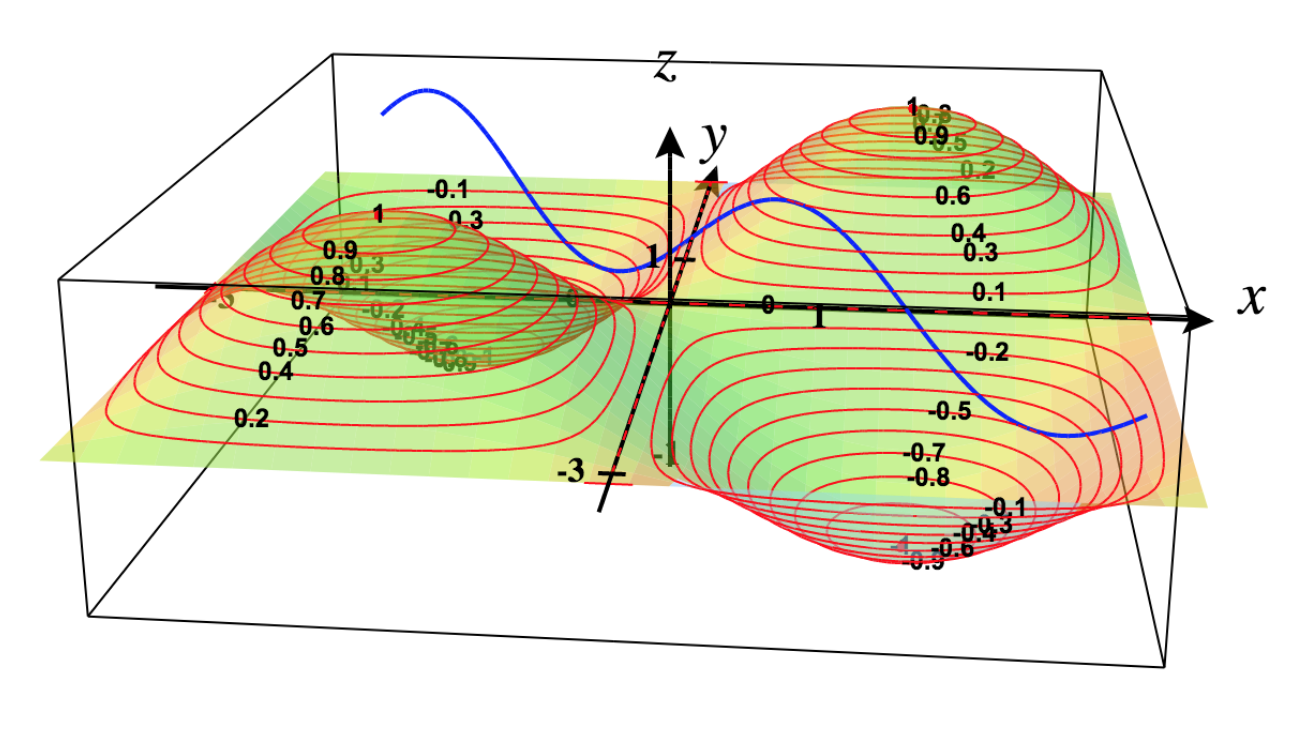
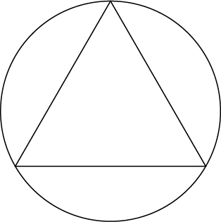
38) Show that, of all the triangles inscribed in a circle of radius \(R\) (see diagram), the equilateral triangle has the largest perimeter.
Contributors
Gilbert Strang (MIT) and Edwin “Jed” Herman (Harvey Mudd) with many contributing authors. This content by OpenStax is licensed with a CC-BY-SA-NC 4.0 license. Download for free at http://cnx.org.
- Paul Seeburger (Monroe Community College) reordered these problems, adding problems 3 and 10 and answers for problems 15 and 17. He also added a full worked-out solution for problem 9 and a link to CalcPlot3D in problems 15, 21 and 35. He also created new images for Problem 37 and expanded the answers for many problems.


