2.3: Graphs of the Tangent and Cotangent Functions

Learning Objectives

• Analyze the graph of \(y=\tan x\).
• Graph variations of \(y=\tan x\).
• Analyze the graph of \(y=\cot x\).
• Graph variations of \(y=\cot x\).

We know the tangent function can be used to find distances, such as the height of a building, mountain, or flagpole. But what if we want to measure repeated occurrences of distance? Imagine, for example, a police car parked next to a warehouse. The rotating light from the police car would travel across the wall of the warehouse in regular intervals. If the input is time, the output would be the distance the beam of light travels. The beam of light would repeat the distance at regular intervals. The tangent function can be used to approximate this distance. Asymptotes would be needed to illustrate the repeated cycles when the beam runs parallel to the wall because, seemingly, the beam of light could appear to extend forever. The graph of the tangent function would clearly illustrate the repeated intervals. In this section, we will explore the graphs of the tangent and cotangent functions. 

Analyzing the Graph of \(y =\tan x\)

We will begin with the graph of the tangent function, plotting points as we did for the sine and cosine functions. Recall that

\[\tan \, x=\dfrac{\sin \, x}{\cos \, x}\]

The period of the tangent function is \(\pi\) because the graph repeats itself on intervals of \(k\pi\) where \(k\) is a constant. If we graph the tangent function on \(−\frac{\pi}{2}\) to \(\frac{\pi}{2}\), we can see the behavior of the graph on one complete cycle. If we look at any larger interval, we will see that the characteristics of the graph repeat.

We can determine whether tangent is an odd or even function by using the definition of tangent.

\[\begin{align*} \tan(-x)&= \dfrac{\sin(-x)}{\cos(-x)} \qquad \text{Definition of tangent}\\[4pt] &= \dfrac{-\sin \, x}{\cos \, x} \qquad \text{Sine is an odd function, cosine is even}\\[4pt] &= -\dfrac{\sin \, x}{\cos \, x} \qquad \text{The quotient of an odd and an even function is odd}\\[4pt] &= -\tan \, x \qquad \text{Definition of tangent} \end{align*}\]

Therefore, tangent is an odd function. We can further analyze the graphical behavior of the tangent function by looking at values for some of the special angles, as listed in Table \(\PageIndex{1}\).

Table \(\PageIndex{1}\)

\(x\)	\(−\dfrac{\pi}{2}\)	\(−\dfrac{\pi}{3}\)	\(−\dfrac{\pi}{4}\)	\(−\dfrac{\pi}{6}\)	0	\(\dfrac{\pi}{6}\)	\(\dfrac{\pi}{4}\)	\(\dfrac{\pi}{3}\)	\(\dfrac{\pi}{2}\)
\(\tan x\)	undefined	\(-\sqrt{3}\)	\(–1\)	\(-\dfrac{\sqrt{3}}{3}\)	0	\(\dfrac{\sqrt{3}}{3}\)	1	\(\sqrt{3}\)	undefined

These points will help us draw our graph, but we need to determine how the graph behaves where it is undefined. If we look more closely at values when \(\frac{\pi}{3}<x<\frac{\pi}{2}\), we can use a table to look for a trend. Because \(\frac{\pi}{3}≈1.05\) and \(\frac{\pi}{2}≈1.57\), we will evaluate \(x\) at radian measures \(1.05<x<1.57\) as shown in Table \(\PageIndex{2}\).

Table \(\PageIndex{2}\)

\(x\)	1.3	1.5	1.55	1.56
\(\tan x\)	3.6	14.1	48.1	92.6

As \(x\) approaches \(\dfrac{\pi}{2}\), the outputs of the function get larger and larger. Because \(y=\tan \, x\) is an odd function, we see the corresponding table of negative values in Table \(\PageIndex{3}\).

Table \(\PageIndex{3}\)

\(x\)	−1.3	−1.5	−1.55	−1.56
\(\tan x\)	−3.6	−14.1	−48.1	−92.6

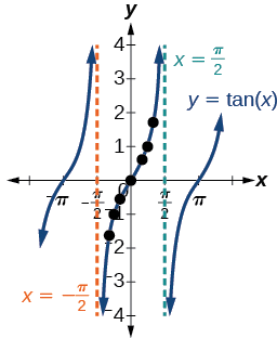
We can see that, as \(x\) approaches \(−\frac{\pi}{2}\), the outputs get smaller and smaller. Remember that there are some values of \(x\) for which \(\cos \, x=0\). For example, \(\cos \left (\frac{\pi}{2} \right)=0\) and \(\cos \left (\frac{3\pi}{2} \right )=0\). At these values, the tangent function is undefined, so the graph of \(y=\tan \, x\) has discontinuities at \(x=\frac{\pi}{2}\) and \(\frac{3\pi}{2}\). At these values, the graph of the tangent has vertical asymptotes. Figure \(\PageIndex{1}\) represents the graph of \(y=\tan \, x\). The tangent is positive from \(0\) to \(\frac{\pi}{2}\) and from \(\pi\) to \(\frac{3\pi}{2}\), corresponding to quadrants I and III of the unit circle.

Figure \(\PageIndex{1}\): Graph of the tangent function

Graphing Variations of \(y = \tan \, x\)

Let's modify the tangent curve by introducing vertical and horizontal stretching and shrinking. As with the sine and cosine functions, the tangent function can be described by a general equation.

\[y=A\tan(Bx) \nonumber\]

We can identify horizontal and vertical stretches and compressions using values of \(A\) and \(B\). The horizontal stretch can typically be determined from the period of the graph. With tangent graphs, it is often necessary to determine a vertical stretch using a point on the graph.

Because there are no maximum or minimum values of a tangent function, the term amplitude cannot be interpreted as it is for the sine and cosine functions. Instead, we will use the phrase stretching/compressing factor when referring to the constant \(A\).

FEATURES OF THE GRAPH OF \(Y = A \tan(Bx)\)

• The stretching factor is \(|A|\).
• The period is \(P=\dfrac{\pi}{|B|}\).
• The domain is all real numbers \(x\),where \(x≠\dfrac{\pi}{2| B |}+\dfrac{π}{| B |}k\) such that \(k\) is an integer.
• The range is \((−\infty,\infty)\).
• To find a pair of asymptotes, solve the equations \(Bx=-\dfrac{\pi}{2}\) and \(Bx=\dfrac{\pi}{2}\). To find other asymptotes from those use the period of the function. 
• \(y=A\tan(Bx)\) is an odd function.

Graphing One Period of a Stretched or Compressed Tangent Function

We can use what we know about the properties of the tangent function to quickly sketch a graph of any stretched and/or compressed tangent function of the form \(f(x)=A\tan(Bx)\). We focus on a single period of the function including the origin, because the periodic property enables us to extend the graph to the rest of the function’s domain if we wish. Our limited domain is then the interval \(\left (−\dfrac{P}{2},\dfrac{P}{2} \right )\) and the graph has vertical asymptotes at \(\pm \dfrac{P}{2}\) where \(P=\dfrac{\pi}{B}\). On \(\left (−\dfrac{\pi}{2},\dfrac{\pi}{2} \right )\), the graph will come up from the left asymptote at \(x=−\dfrac{\pi}{2}\), cross through the origin, and continue to increase as it approaches the right asymptote at \(x=\dfrac{\pi}{2}\). To make the function approach the asymptotes at the correct rate, we also need to set the vertical scale by actually evaluating the function for at least one point that the graph will pass through.

Given the function \(f(x)=A \tan(Bx)\), graph one period.

1. Identify the stretching factor, \(| A |\).
2. Identify B and determine the period, \(P=\dfrac{\pi}{| B |}\).
3. To find a pair of asymptotes, solve the equations \(Bx=-\dfrac{\pi}{2}\) and \(Bx=\dfrac{\pi}{2}\). To find other asymptotes from those use the period of the function. 
4. For \(A>0\), the curve increases in between a pair of asymptotes. For \(A<0\) the curve decreases in between a pair of asymptotes. 

Example \(\PageIndex{1}\): Sketching a Compressed Tangent

Sketch a graph of one period of the function \(y=0.5\tan \left (\dfrac{\pi}{2}x \right )\).

Solution

First, we identify \(A\) and \(B\).

Figure \(\PageIndex{2}\)

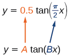
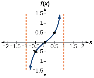
Because \(A=0.5\) and \(B=\dfrac{\pi}{2}\), we can find the stretching/compressing factor and period. The period is \(\dfrac{\pi}{\dfrac{\pi}{2}}=2\). To find a pair of asymptotes we solve the equations \(\dfrac{\pi}{2}x=-\dfrac{\pi}{2}\) and \(\dfrac{\pi}{2}x=\dfrac{\pi}{2}\), which give solutions of \(x=-1\) and \(x=1\), so we know at those two locations we will have vertical asymptotes. At a quarter period from the origin, we have

\[\begin{align*} f(0.5)&= 0.5\tan \left (\dfrac{0.5\pi}{2} \right )\\[4pt] &= 0.5\tan \left (\dfrac{\pi}{4} \right )\\[4pt] &= 0.5 \end{align*}\]

This means the curve must pass through the points \((0.5,0.5)\), \((0,0)\),and \((−0.5,−0.5)\). The only inflection point is at the origin. Figure \(\PageIndex{3}\) shows the graph of one period of the function.

Figure \(\PageIndex{3}\)

Exercise \(\PageIndex{1}\)

Sketch a graph of \(f(x)=3\tan \left (\dfrac{\pi}{6}x \right )\).

Answer

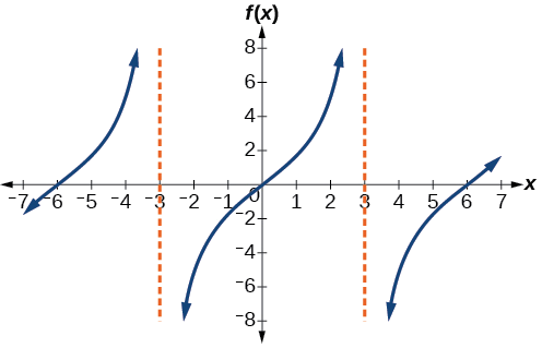
Figure \(\PageIndex{4}\)

Graphing One Period of a Shifted Tangent Function

Now that we can graph a tangent function that is stretched or compressed, we will add a vertical and/or horizontal (or phase) shift. In this case, we add \(C\) and \(D\) to the general form of the tangent function.

\[f(x)=A\tan(Bx−C)+D \nonumber\]

The graph of a transformed tangent function is different from the basic tangent function \(\tan x\) in several ways:

FEATURES OF THE GRAPH OF \(Y = A\tan(Bx−C)+D\)

• The stretching factor is \(| A |\).
• The period is \(\dfrac{\pi}{| B |}\).
• The domain is \(x≠\dfrac{C}{B}+\dfrac{\pi}{| B |}k\),where \(k\) is an integer.
• The range is \((−∞,−| A |]∪[| A |,∞)\).
• To find a pair of asymptotes, solve the equations \(Bx-C=-\dfrac{\pi}{2}\) and \(Bx-C=\dfrac{\pi}{2}\)
• There is no amplitude.
• The "wiggle" point of the curve will happen on the horizontal line \(y=D\)
• \(y=A \tan(Bx)\) is and odd function because it is the quotient of odd and even functions (sin and cosine respectively).

Howto: Given the function \(y=A\tan(Bx−C)+D\), sketch the graph of one period.

1. Express the function given in the form \(y=A\tan(Bx−C)+D\).
2. Identify the stretching/compressing factor, \(| A |\).
3. Identify \(B\) and determine the period, \(P=\dfrac{\pi}{|B|}\).
4. Solve the equations \(Bx-C=-\dfrac{\pi}{2}\) and \(Bx-C=\dfrac{\pi}{2}\) to find a pair of asymptotes
5. Plot any three reference points and draw the graph through these points.

Example \(\PageIndex{2}\): Graphing One Period of a Shifted Tangent Function

Graph one period of the function \(y=−2\tan(\pi x+\pi)−1\).

Solution

• Step 1. The function is already written in the form \(y=A\tan(Bx−C)+D\).
• Step 2. \(A=−2\), so the stretching factor is \(|A|=2\). Because of the negative, this curve will be reflected across the \(x\)-axis compared to the curve of \(y=tanx\), which means the curve will be decreasing in between each pair of asymptotes. 
• Step 3. \(B=\pi\), so the period is \(P=\dfrac{\pi}{| B |}=\dfrac{\pi}{\pi}=1\).
• Step 4. Solve the equations \(\pi x+\pi=-\dfrac{\pi}{2}\) and \(\pi x+\pi=\dfrac{\pi}{2}\). For the first equation: 

\[\begin{align*} \pi x+\pi&=-\dfrac{\pi}{2} \\ \pi x&=-\dfrac{\pi}{2}-\pi \\ \pi x&=-\dfrac{\pi}{2}-\dfrac{2\pi}{2} \\ \pi x&=-\dfrac{3\pi}{2} \\ x&=-\dfrac{3\pi}{2\pi} \\ x&=-\dfrac{3}{2} \end{align*} \]

Similarly, for the second equation we have: 

\[\begin{align*} \pi x+\pi&=\dfrac{\pi}{2} \\ \pi x&=\dfrac{\pi}{2}-\pi \\ \pi x&=\dfrac{\pi}{2}-\dfrac{2\pi}{2} \\ \pi x&=-\dfrac{\pi}{2} \\ x&=-\dfrac{\pi}{2\pi} \\ x&=-\dfrac{1}{2} \end{align*} \]

• Step 5. We can divide the distance of the period by 4 to find three points in between the asymptotes. Taking 1 divided by 4 we have \(\dfrac{1}{4}\) or 0.25. Our asymptotes are at -1.5 and -0.5. Starting at the left asymptote -1.5 and increasing by 0.25 we land on the values -1.25, -1, and -0.75. Plugging these values in for \(x\) gives us the points \((−1.25,1)\), \((−1,−1)\), and \((−0.75,−3)\). The graph is shown in Figure \(\PageIndex{5}\).

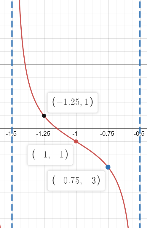
Figure \(\PageIndex{5}\)

Analysis

Note that this is a decreasing function because \(A<0\).

Exercise \(\PageIndex{2}\)

How would the graph in Example \(\PageIndex{2}\) look different if we made \(A=2\) instead of \(−2\)?

Answer

It would be reflected across the line \(y=−1\), becoming an increasing function.

Example \(\PageIndex{3}\): Identifying the Graph of a Stretched Tangent

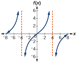
Find a formula for the function graphed in Figure \(\PageIndex{6}\).

Figure \(\PageIndex{6}\): A stretched tangent function

Solution

The graph has the shape of a tangent function.

• Step 1. One cycle extends from \(–4\) to \(4\), so the period is \(P=8\). Since \(P=\dfrac{\pi}{| B |}\), we have \(B=\dfrac{π}{P}=\dfrac{\pi}{8}\).
• Step 2. The equation must have the form \(f(x)=A\tan \left (\dfrac{\pi}{8}x \right )\).
• Step 3. To find the vertical stretch \(A\),we can use the point \((2,2)\). \[\begin{align*} 2&=A\tan \left (\dfrac{\pi}{8}\cdot 2 \right )\\[4pt] &=A\tan \left (\dfrac{\pi}{4} \right ) \end{align*}\]

Because \(\tan \left (\dfrac{\pi}{4} \right )=1\), \(A=2\).

This function would have a formula \(f(x)=2\tan \left (\dfrac{\pi}{8}x \right )\).

Exercise \(\PageIndex{3}\)

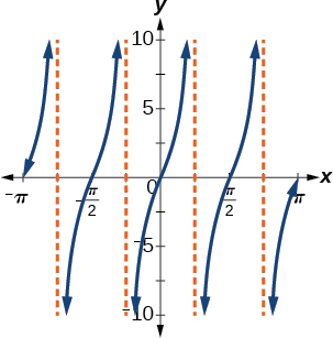
Find a formula for the function in Figure \(\PageIndex{7}\).

Figure \(\PageIndex{7}\)

Answer

\(g(x)=4\tan(2x)\)

Analyzing the Graph of \(y = \cot x\)

The last trigonometric function we need to explore is cotangent. The cotangent is defined by the reciprocal identity \(cot \, x=\dfrac{1}{\tan x}\). Notice that the function is undefined when the tangent function is \(0\), leading to a vertical asymptote in the graph at \(0\), \(\pi\), etc. Since the output of the tangent function is all real numbers, the output of the cotangent function is also all real numbers.

We can graph \(y=\cot x\) by observing the graph of the tangent function because these two functions are reciprocals of one another. See Figure \(\PageIndex{8}\). Where the graph of the tangent function decreases, the graph of the cotangent function increases. Where the graph of the tangent function increases, the graph of the cotangent function decreases.

The cotangent graph has vertical asymptotes at each value of \(x\) where \(\tan x=0\); we show these in the graph below with dashed lines. Since the cotangent is the reciprocal of the tangent, \(\cot x\) has vertical asymptotes at all values of \(x\) where \(\tan x=0\), and \(\cot x=0\) at all values of \(x\) where \(\tan x\) has its vertical asymptotes.

Figure \(\PageIndex{8}\): The cotangent function

FEATURES OF THE GRAPH OF \(Y = A \cot(BX)\)

• The stretching factor is \(|A|\).
• The period is \(P=\dfrac{\pi}{|B|}\).
• The domain is \(x≠\dfrac{\pi}{|B|}k\), where \(k\) is an integer.
• The range is \((−∞,∞)\).
• The asymptotes occur at \(x=\dfrac{\pi}{| B |}k\), where \(k\) is an integer.
• \(y=A\cot(Bx)\) is an odd function.

Graphing Variations of \(y =\cot x\)

We can transform the graph of the cotangent in much the same way as we did for the tangent. The equation becomes the following.

\[y=A\cot(Bx−C)+D\]

PROPERTIES OF THE GRAPH OF \(Y = A \cot(Bx-C)+D\)

• The stretching factor is \(| A |\).
• The period is \(\dfrac{\pi}{|B|}\)
• The domain is \(x≠\dfrac{C}{B}+\dfrac{\pi}{| B |}k\),where \(k\) is an integer.
• The range is \((−∞,−|A|]∪[|A|,∞)\).
• A pair of vertical asymptotes occur at the solutions of the equations \(Bx-C=0\) and \(Bx-C=\pi\). To find others, use the distance of the period. 
• There is no amplitude.
• \(y=A\cot(Bx)\) is an odd function because it is the quotient of even and odd functions (cosine and sine, respectively)

Example \(\PageIndex{4}\): Graphing Variations of the Cotangent Function

Determine the stretching factor, period, and phase shift of \(y=3\cot(4x)\), and then sketch a graph.

Solution

• Step 1.  The stretching factor is \(|A|=3\).
• Step 2. The period is \(P=\dfrac{\pi}{4}\). Dividing this by 4 gives \(\dfrac{\pi}{16}\). Every time we travel a distance of \(\dfrac{\pi}{16}\) we will be at a vertical asymptote, a wiggle point, or a point on either side of the wiggle point.
• Step 3. To find a pair of vertical asymptotes, we solve the equations \(4x=0\) and \(4x=\pi\), which give solutions \(x=0\) and \(x=\dfrac{\pi}{4}\)
• Step 4. Plot points in between the vertical asymptotes. Three such points are \(\left (\dfrac{\pi}{16},3 \right )\), \(\left (\dfrac{\pi}{8},0 \right )\) \(\left (\dfrac{3\pi}{16},−3 \right )\).

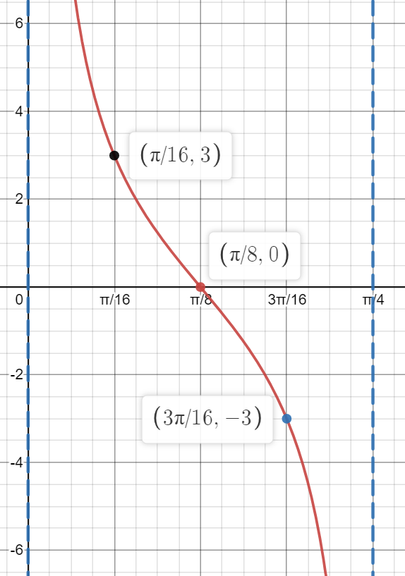
Figure \(\PageIndex{9}\)

Given a modified cotangent function of the form \(f(x)=A\cot(Bx−C)+D\), graph one period.

1. Identify the stretching factor, \(| A |\). If \(A>0\) the function is decreasing in between a pair of asymptotes. If \(A<0\) then it is increasing. 
2. Identify the period, \(P=\dfrac{\pi}{|B|}\).
3. Find a pair of asymptotes by solving the equations \(Bx-C=0\) and \(Bx-C=\pi\). To find others, use the distance of the period. 
4. Plot any three reference points and draw the graph through these points. Points that will be nice to work with are those a distance of a quarter of the period away from the asymptotes and in the center of the asymptotes. In the center of the asymptotes is where you should have your wiggle point. The wiggle point will be on the line \(y=D\) 

Example \(\PageIndex{5}\): Graphing a Modified Cotangent

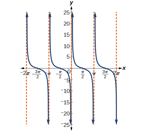
Sketch a graph of one period of the function \(f(x)=4\cot \left (\dfrac{\pi}{8}x−\dfrac{\pi}{2} \right )−2\).

Solution

• Step 1. \(A=4\),so the stretching factor is \(4\).
• Step 2. \(B=\dfrac{\pi}{8}\), so the period is \(P=\dfrac{\pi}{| B |}=\dfrac{\pi}{\dfrac{\pi}{8}}=8\).
• Step 3. To find a pair of asymptotes we solve the equations \(\dfrac{\pi}{8}x−\dfrac{\pi}{2}=0\) and \(\dfrac{\pi}{8}x−\dfrac{\pi}{2}=\pi\). For the first equation: 

\[ \begin{align*} \dfrac{\pi}{8}x−\dfrac{\pi}{2}&=0 \\ \dfrac{\pi}{8}x&=\dfrac{\pi}{2} \\ x&=\dfrac{\dfrac{\pi}{2}}{\dfrac{\pi}{8}} \\ x&=\dfrac{\pi}{2} \times \dfrac{8}{\pi} \\ x&=4 \end{align*} \]

For the second equation: 

\[ \begin{align*} \dfrac{\pi}{8}x−\dfrac{\pi}{2}&=\pi \\ \dfrac{\pi}{8}x&=\pi + \dfrac{\pi}{2} \\ \dfrac{\pi}{8}x&=\dfrac{2\pi}{2} + \dfrac{\pi}{2} \\ \dfrac{\pi}{8}x&=\dfrac{3\pi}{2} \\ x&=\dfrac{\dfrac{3\pi}{2}}{\dfrac{\pi}{8}} \\ x&=\dfrac{3\pi}{2} \times \dfrac{8}{\pi} \\ x&=12 \end{align*} \]

The vertical asymptotes are located at \(x=4\) and \(x=12\)

• Step 4. Dividing the period 8 by 4 gives 2. Every 2 units we will hit an asymptote, wiggle point, or a point on either side of the wiggle point. The wiggle point will happen half way between the asymptotes on the line \(y=-2\). Starting at the left asymptote and increasing by 2 gives the values 6, 8, and 10. Three points we can use to guide the graph are \((6,2)\), \((8,−2)\), and \((10,−6)\). 

The graph is shown in Figure \(\PageIndex{10}\).

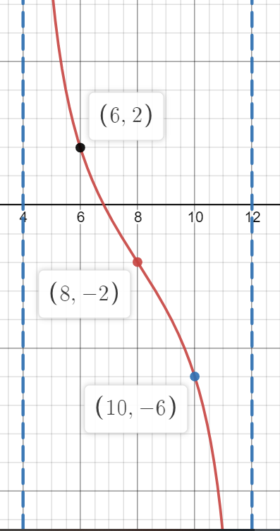
Figure \(\PageIndex{10}\): One period of a modified cotangent function

Using the Graphs of Trigonometric Functions to Solve Real-World Problems

Many real-world scenarios represent periodic functions and may be modeled by trigonometric functions. As an example, let’s return to the scenario from the section opener. Have you ever observed the beam formed by the rotating light on a police car and wondered about the movement of the light beam itself across the wall? The periodic behavior of the distance the light shines as a function of time is obvious, but how do we determine the distance? We can use the tangent function.

Example \(\PageIndex{6}\): Using Trigonometric Functions to Solve Real-World Scenarios

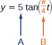
Suppose the function \(y=5\tan(\dfrac{\pi}{4}t)\) marks the distance in the movement of a light beam from the top of a police car across a wall where \(t\) is the time in seconds and \(y\) is the distance in feet from a point on the wall directly across from the police car.

1. Find and interpret the stretching factor and period.
2. Graph on the interval \([0,5]\).
3. Evaluate \(f(1)\) and discuss the function’s value at that input.

Solution

1. We know from the general form of \(y=A\tan(Bt)\) that \(| A |\) is the stretching factor and \(\dfrac{\pi}{B}\) is the period.

Figure \(\PageIndex{11}\)

We see that the stretching factor is \(5\). This means that the beam of light will have moved \(5\) ft after half the period.

The period is \(\dfrac{\pi}{\tfrac{\pi}{4}}=\dfrac{\pi}{1}⋅\dfrac{4}{\pi}=4\). This means that every \(4\) seconds, the beam of light sweeps the wall. The distance from the spot across from the police car grows larger as the police car approaches.

2. To graph the function, we draw an asymptote at \(t=2\) and use the stretching factor and period. See Figure \(\PageIndex{12}\)

Figure \(\PageIndex{12}\)

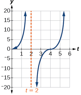
3. period: \(f(1)=5\tan(\frac{\pi}{4}(1))=5(1)=5\); after \(1\) second, the beam of has moved \(5\) ft from the spot across from the police car.

Key Equations

Shifted, compressed, and/or stretched tangent function

\(y=A \tan(Bx−C)+D\)

Shifted, compressed, and/or stretched cotangent function

\(y=A \cot(Bx−C)+D\)

Key Concepts

• The tangent function has period \(π\).
• \(f( x )=A\tan( Bx−C )+D\) is a tangent with vertical and/or horizontal stretch/compression and shift. 
• The cotangent function has period \(\pi\) and vertical asymptotes at \(0,±\pi,±2\pi\),....
• The range of cotangent is \(( −∞,∞ )\), and the function is decreasing at each point in its range.
• The cotangent is zero at \(±\dfrac{\pi}{2},±\dfrac{3\pi}{2}\),....
• \(f(x)=A\cot(Bx−C)+D\) is a cotangent with vertical and/or horizontal stretch/compression and shift.
• Real-world scenarios can be solved using graphs of trigonometric functions.