4.5: Geometric Meaning of Scalar Multiplication

Last updated
Save as PDF

Page ID: 72196

\( \newcommand{\vecs}[1]{\overset { \scriptstyle \rightharpoonup} {\mathbf{#1}} } \) \( \newcommand{\vecd}[1]{\overset{-\!-\!\rightharpoonup}{\vphantom{a}\smash {#1}}} \)\(\newcommand{\id}{\mathrm{id}}\) \( \newcommand{\Span}{\mathrm{span}}\) \( \newcommand{\kernel}{\mathrm{null}\,}\) \( \newcommand{\range}{\mathrm{range}\,}\) \( \newcommand{\RealPart}{\mathrm{Re}}\) \( \newcommand{\ImaginaryPart}{\mathrm{Im}}\) \( \newcommand{\Argument}{\mathrm{Arg}}\) \( \newcommand{\norm}[1]{\| #1 \|}\) \( \newcommand{\inner}[2]{\langle #1, #2 \rangle}\) \( \newcommand{\Span}{\mathrm{span}}\) \(\newcommand{\id}{\mathrm{id}}\) \( \newcommand{\Span}{\mathrm{span}}\) \( \newcommand{\kernel}{\mathrm{null}\,}\) \( \newcommand{\range}{\mathrm{range}\,}\) \( \newcommand{\RealPart}{\mathrm{Re}}\) \( \newcommand{\ImaginaryPart}{\mathrm{Im}}\) \( \newcommand{\Argument}{\mathrm{Arg}}\) \( \newcommand{\norm}[1]{\| #1 \|}\) \( \newcommand{\inner}[2]{\langle #1, #2 \rangle}\) \( \newcommand{\Span}{\mathrm{span}}\)\(\newcommand{\AA}{\unicode[.8,0]{x212B}}\)

Outcomes

Understand scalar multiplication, geometrically.

Recall that the point \(P=\left( p_{1},p_{2},p_{3}\right)\) determines a vector \(\vec{p}\) from \(0\) to \(P\). The length of \(\vec{p}\), denoted \(\| \vec{p} \|\), is equal to \(\sqrt{p_{1}^{2}+p_{2}^{2}+p_{3}^{2}}\) by Definition 4.4.1.

Now suppose we have a vector \(\vec{u} = \left[ \begin{array}{lll} u_1 & u_2 & u_3 \end{array} \right]^T\) and we multiply \(\vec{u}\) by a scalar \(k\). By Definition 4.2.2, \(k\vec{u} = \left[ \begin{array}{rrr} ku_{1} & ku_{2} & ku_{3} \end{array} \right]^T\). Then, by using Definition 4.4.1, the length of this vector is given by \[\sqrt{\left( \left( k u_{1}\right) ^{2}+\left( k u_{2}\right) ^{2}+\left( k u_{3}\right) ^{2}\right) }=\left\vert k \right\vert \sqrt{u_{1}^{2}+u_{2}^{2}+u_{3}^{2}}\nonumber \] Thus the following holds. \[\| k \vec{u} \| =\left\vert k \right\vert \| \vec{u} \|\nonumber \] In other words, multiplication by a scalar magnifies or shrinks the length of the vector by a factor of \(\left\vert k \right\vert\). If \(\left\vert k \right\vert > 1\), the length of the resulting vector will be magnified. If \(\left\vert k \right\vert <1\), the length of the resulting vector will shrink. Remember that by the definition of the absolute value, \(\left\vert k \right\vert >0\).

What about the direction? Draw a picture of \(\vec{u}\) and \(k\vec{u}\) where \(k\) is negative. Notice that this causes the resulting vector to point in the opposite direction while if \(k >0\) it preserves the direction the vector points. Therefore the direction can either reverse, if \(k < 0\), or remain preserved, if \(k > 0\).

Consider the following example.

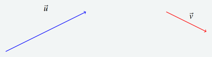
Example \(\PageIndex{1}\): Graphing Scalar Multiplication

Consider the vectors \(\vec{u}\) and \(\vec{v}\) drawn below.

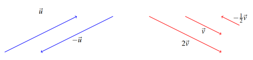
Draw \(-\vec{u}\), \(2\vec{v}\), and \(-\frac{1}{2}\vec{v}\).

Solution

In order to find \(-\vec{u}\), we preserve the length of \(\vec{u}\) and simply reverse the direction. For \(2\vec{v}\), we double the length of \(\vec{v}\), while preserving the direction. Finally \(-\frac{1}{2}\vec{v}\) is found by taking half the length of \(\vec{v}\) and reversing the direction. These vectors are shown in the following diagram.

Now that we have studied both vector addition and scalar multiplication, we can combine the two actions. Recall Definition 9.2.2 of linear combinations of column matrices. We can apply this definition to vectors in \(\mathbb{R}^n\). A linear combination of vectors in \(\mathbb{R}^n\) is a sum of vectors multiplied by scalars.

In the following example, we examine the geometric meaning of this concept.

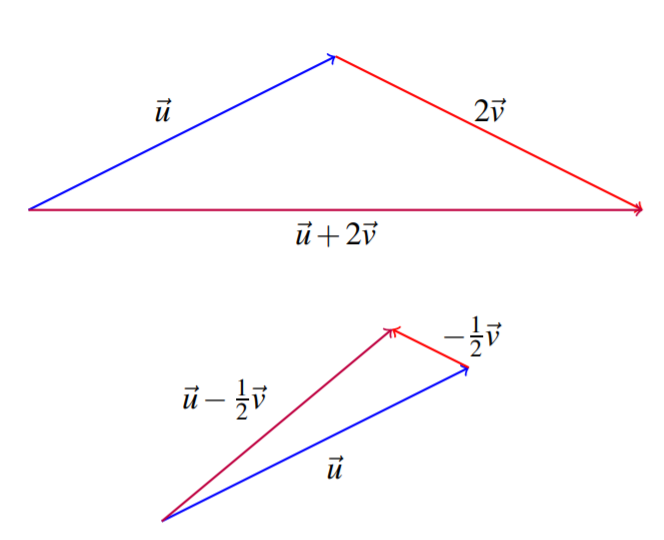
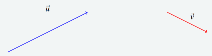
Example \(\PageIndex{2}\): Graphing a Linear Combination of Vectors

Consider the following picture of the vectors \(\vec{u}\) and \(\vec{v}\)

Sketch a picture of \(\vec{u}+2\vec{v},\vec{u}-\frac{1}{2}\vec{v}.\)

Solution

The two vectors are shown below.