5.9.3: Transportation Networks and Flows
- Page ID
- 18878
investigate!
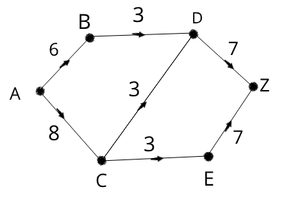
At the end of the school day, all the students plan on driving from school (vertex A) to the concert (at vertex Z). The directed edges in the graph below represent one-way roads, and the weight of each edge represents the number of vehicles (in hundreds) that particular road can handle in one hour. What is the greatest number of vehicles that can get from school to the concert in one hour? How many vehicles should take each road?
Definition
A transportation network is a connected, weighted, directed graph with the following properties.
- There is one source, a vertex with no incoming edges. [In other language, the vertex has indegree 0.]
- There is one sink, a vertex with no outgoing edges. [In other language, the vertex has outdegree 0.]
- Each edge \((u,v)\) is assigned a nonnegative weight \(C_{uv}\) called the capacity of that edge. [Notice I wrote the edge as an ordered pair rather than a set. This is because each edge has an initial vertex and a terminal vertex, so the order matters.]
Transportation networks can also be used to model oil flowing through a series of pipelines, data flowing through a network of computers, and many other situations.
Definition
Let \(G\) be a transportation network with capacity \(C_{ij}\) on edge \((i,j)\). A flow \(F\) on \(G\) assigns to each edge \((i,j)\) a nonnegative number \(F_{ij}\), called the flow on edge \((i,j)\) with the following properties.
- \(F_{ij}\leq C_{ij}\).
- For every vertex \(i\) other than the source or the sink, \(\sum_j F_{ij}=\sum_j F_{ji}\).
What do these two conditions mean in words? The first says that the flow cannot exceed the capacity on an edge. We can see why this condition is necessary - we cannot, for example, send more oil through a pipeline than it can handle. The second says that the flow IN to a vertex must be equal to the flow OUT of that same vertex (except at the source or the sink). Again this condition makes sense: if oil is flowing through a series of pipelines, we should not gain or lose oil between the source of the oil and location to which we are sending it.
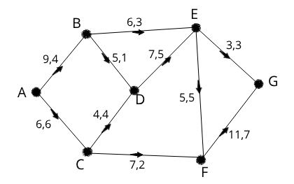
To write a flow on a transportation network, give each edge a pair of numbers with the capacity of an edge preceding the flow along that edge: \(C_{ij},F_{ij}\). Express your solution to the initial example in this section as a flow on a transportation network.
Theorem \(\PageIndex{1}\)
For any flow \(F\) on a transportation network, the flow out of the source must equal the flow into the sink. In symbols, \(\sum_j F_{aj}=\sum_j F_{jz}\).
- Proof
-
This proof is left as an exercise.
Because of the previous theorem, we can make the following definition.
Definition
The value of a flow is the total flow out of the sink (or into the source). A maximal flow is a flow with greatest possible value.
Definition
A cut in a transportation network \(G\) is a partition of the vertices of \(G\) into two sets \(S\) and \(T\) so that the source is in \(S\) and the sink is in \(T\).
For example \(S=\{A,B\}\) and \(T=\{C,D,E,Z\}\) is a cut for the transportation network at the beginning of the section.
Definition
The capacity of the cut S,T is the sum of the capacities of all edges starting at a vertex in \(S\) and ending at a vertex in \(T\). Equivalently, it is the number \(\sum_{i\in S, j\in T} C_{ij}\). A minimal cut is a cut with the least possible capacity.
The capacity of the previous cut is \(3+8=11\). A minimal cut for the same network is \(S=\{A,B,C\}\) and \(T=\{D,E,Z\}\). This cut has capacity 9.
It turns out that maximal flows are related to minimal cuts.
Theorem \(\PageIndex{2}\)
Let \(F\) be a flow on a transportation network \(G\) and let \(S,T\) be a cut. If \(\sum_i F_{ai}=\sum_{i\in S, j\in T} C_{ij}\) (i.e. if the value of the flow is equal to the capacity of the cut), then the flow is maximal and the cut is minimal.
- Proof
-
The proof is omitted.
We present below an algorithm that can be used to find a maximal flow in a transportation network. It is given below in sentences rather than in pseudocode for ease of understanding. The basic idea is that we begin with a flow of zero along each edge. We use the algorithm to find a path from the source to the sink along which we can increase the flow. We do so, and then we try again. We keep doing so until we cannot anymore; what we are left with is a maximal flow. The proof that the algorithm produces a maximal flow and a minimum cut are omitted.
Max Flow algorithm
- Label the source \((source,+,\infty)\).
-
Look at a labeled vertex. Suppose it is called \(v\) and has label \((u, \pm, a)\). For each unlabeled vertex \(w\) do the following:
-
If there is an edge from \(v\) to \(w\), and the current flow from \(v\) to \(w\) is below capacity, give \(w\) the label \((v,+,b)\) where \(b\) is either \(a\) or the capacity minus the flow, whichever is smaller.
-
If there is an edge from \(w\) to \(v\) and the current flow from \(w\) to \(v\) is positive, then give \(w\) the label \((v,-,b)\) where \(b\) is either \(a\) or the current flow, whichever is smaller.
-
Otherwise, don't give \(w\) a label.
-
-
Repeat step 2 until the sink is labeled or you can't label anymore.
-
If the sink is labeled, increase the flow by the amount in the label on the sink, following the path back to the source. Notice that if you encounter any “-” you need to decrease the flow on that arc. Then start again at step 1 with this new flow.
-
If the sink isn’t labeled you are done. The current flow is maximal. We have also found a minimal cut: the set of labeled vertices is S and the set of unlabeled vertices is T.
-
Exercise \(\PageIndex{3}\)
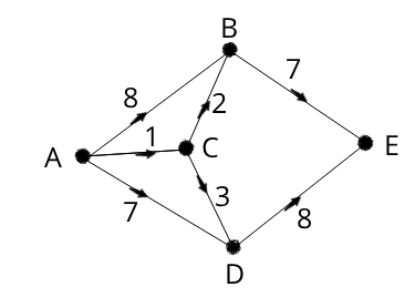
Use the max flow algorithm to determine a maximal flow, the value of the maximal flow, and a minimal cut for the transportation network below.
Use the max flow algorithm to determine a maximal flow, the value of the maximal flow, and a minimal cut for the transportation network with the given flow below.