
5.8: Trees
- Page ID
- 18835
Investigate!
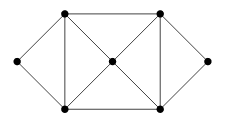
Consider the graph drawn below.

- Find a subgraph with the smallest number of edges that is still connected and contains all the vertices.
- Find a subgraph with the largest number of edges that doesn't contain any cycles.
- What do you notice about the number of edges in your examples above? Is this a coincidence?
Definition
A tree is a connected graph with no cycles. (Alternatively, a tree is a connected acyclic graph.)
A forest is a graph containing no cycles. Note that this means a connected forest is a tree.
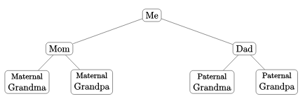
So far so good, but while your grandparents are (probably) not blood-relatives, if we go back far enough, it is likely that they did have some common ancestor. If you trace the tree back from you to that common ancestor, then down through your other grandparent, you would have a cycle, and thus the graph would not be a tree.
You might also have seen something called a decision tree before (for example when deciding whether a series converges or diverges). Sometimes these too contain cycles, as the decision for one node might lead you back to a previous step.
Both the examples of trees above also have another feature worth mentioning: there is a clear order to the vertices in the tree. In general, there is no reason for a tree to have this added structure, although we can impose such a structure by considering rooted trees, where we simply designate one vertex as the root. We will consider such trees in more detail later in this section.
Properties of Trees
We wish to really understand trees. This means we should discover properties of trees; what makes them special and what is special about them.
A tree is an connected graph with no cycles. Is there anything else we can say? It would be nice to have other equivalent conditions for a graph to be a tree. That is, we would like to know whether there are any graph theoretic properties that all trees have, and perhaps even that only trees have.
To get a feel for the sorts of things we can say, we will consider three propositions about trees. These will also illustrate important proof techniques that apply to graphs in general, and happen to be a little easier for trees.
Our first proposition gives an alternate definition for a tree. That is, it gives necessary and sufficient conditions for a graph to be a tree.
Proposition \(\PageIndex{1}\)
A graph T is a tree if and only if between every pair of distinct vertices there is a unique path.
- Proof
-
This is an “if and only if” statement, so we must prove two implications. We start by proving that if T is a tree, then between every pair of distinct vertices there is a unique path.
Assume T is a tree, and let \(u\) and \(v\) be distinct vertices (if T only has one vertex, then the conclusion is satisfied automatically). We must show two things to show that there is a unique path between \(u\) and \(v\): that there is a path, and that there is not more than one path. The first of these is automatic, since T is a tree, it is connected, so there is a path between any pair of vertices.
To show the path is unique, we suppose there are two paths between \(u\) and \(v\), and get a contradiction. The two paths might start out the same, but since they are different, there is some first vertex \(u′\) after which the two paths diverge. However, since the two paths both end at \(v\), there is some first vertex after \(u′\) that they have in common, call it \(v′\). Now consider the two paths from \(u′\) to \(v′\). Taken together, these form a cycle, which contradicts our assumption that T is a tree.
Now we consider the converse: if between every pair of distinct vertices of T there is a unique path, then T is a tree. So assume the hypothesis: between every pair of distinct vertices of T there is a unique path. To prove that T is a tree, we must show it is connected and contains no cycles.
The first half of this is easy: T is connected, because there is a path between every pair of vertices. To show that T has no cycles, we assume it does, for the sake of contradiction. Let \(u\) and \(v\) be two distinct vertices in a cycle of T. Since we can get from \(u\) to \(v\) by going clockwise or counterclockwise around the cycle, there are two paths from \(u\) and \(v\), contradicting our assumption.
We have established both directions so we have completed the proof.
Read the proof above very carefully. Notice that both directions had two parts: the existence of paths, and the uniqueness of paths (which related to the fact there were no cycles). In this case, these two parts were really separate. In fact, if we just considered graphs with no cycles (a forest), then we could still do the parts of the proof that explore the uniqueness of paths between vertices, even if there might not exist paths between vertices.
This observation allows us to state the following corollary:
Corollary \(\PageIndex{2}\)
A graph is a forest if and only if there is at most one path between every pair of vertices.
Proposition \(\PageIndex{3}\)
Any tree with at least two vertices has at least two vertices of degree one.
- Proof
-
We give a proof by contradiction. Let T be a tree with at least two vertices, and suppose, contrary to stipulation, that there are not two vertices of degree one.
Let \(P\) be a path in T of longest possible length. Let \(u\) and \(v\) be the endpoints of the path. Since T does not have two vertices of degree one, at least one of these must have degree two or higher. Say that it is \(u\). We know that \(u\) is adjacent to a vertex in the path \(P\), but now it must also be adjacent to another vertex, call it \(u′\).
Where is \(u′\)? It cannot be a vertex of \(P\), because if it was, there would be two distinct paths from \(u\) to \(u′\): the edge between them, and the first part of \(P\) (up to \(u′\)). But \(u′\) also cannot be outside of \(P\), for if it was, there would be a path from \(u′\) to \(v\) that was longer than \(P\), which has longest possible length.
This contradiction proves that there must be at least two vertices of degree one. In fact, we can say a little more: \(u\) and \(v\) must both have degree one.
The proposition is quite useful when proving statements about trees, because we often prove statements about trees by induction. To do so, we need to reduce a given tree to a smaller tree (so we can apply the inductive hypothesis). Getting rid of a vertex of degree one is an obvious choice, and now we know there is always one to get rid of.
To illustrate how induction is used on trees, we will consider the relationship between the number of vertices and number of edges in trees. Is there a tree with exactly 7 vertices and 7 edges? Try to draw one? Could a tree with 7 vertices have only 5 edges? There is a good reason that these seem impossible to draw.
Proposition \(\PageIndex{4}\)
Let T be a tree with \(v\) vertices and \(e\) edges. Then \(e=v-1\).
- Proof
-
We will give a proof by induction on the number of vertices in the tree. That is, we will prove that every tree with \(v\) vertices has exactly \(v−1\) edges, and then use induction to show this is true for all \(v\geq 1.\)
For the base case, consider all trees with \(v=1\) vertices. There is only one such tree: the graph with a single isolated vertex. This graph has \(e=0\) edges, so we see that \(e=v−1\) as needed.
Now for the inductive case, fix \(k\geq 1\) and assume that all trees with \(v=k\) vertices have exactly \(e=k−1\) edges. Now consider an arbitrary tree T with \(v=k+1\) vertices. By Proposition 3, T has a vertex \(v_0\) of degree one. Let T′ be the tree resulting from removing \(v_0\) from T (together with its incident edge). Since we removed a leaf, T′ is still a tree (the unique paths between pairs of vertices in T′ are the same as the unique paths between them in T).
Now T′ has \(k\) vertices, so by the inductive hypothesis, has \(k−1\) edges. What can we say about T? Well, it has one more edge than T′, so it has \(k\) edges. But this is exactly what we wanted: \(v=k+1\), \(e=k\) so indeed \(e=v−1\). This completes the proof.
There is a very important feature of this induction proof that is worth noting. Induction makes sense for proofs about graphs because we can think of graphs as growing into larger graphs. However, this does NOT work. It would not be correct to start with a tree with \(k\) vertices, and then add a new vertex and edge to get a tree with \(k+1\) vertices, and note that the number of edges also grew by one. Why is this bad? Because how do you know that every tree with \(k+1\) vertices is the result of adding a vertex to your arbitrary starting tree? You don't!
The point is that whenever you give an induction proof that a statement about graphs that holds for all graphs with \(v\) vertices, you must start with an arbitrary graph with \(v+1\) vertices, then reduce that graph to a graph with \(v\) vertices, to which you can apply your inductive hypothesis.
Rooted Trees
So far, we have thought of trees only as a particular kind of graph. However, it is often useful to add additional structure to trees to help solve problems. Data is often structured like a tree. This book, for example, has a tree structure: draw a vertex for the book itself. Then draw vertices for each chapter, connected to the book vertex. Under each chapter, draw a vertex for each section, connecting it to the chapter it belongs to. The graph will not have any cycles; it will be a tree. But a tree with clear hierarchy which is not present if we don't identify the book itself as the “top”.
As soon as one vertex of a tree is designated as the root, then every other vertex on the tree can be characterized by its position relative to the root. This works because between any two vertices in a tree, there is a unique path. So from any vertex, we can travel back to the root in exactly one way. This also allows us to describe how distinct vertices in a rooted tree are related.
If two vertices are adjacent, then we say one of them is the parent of the other, which is called the child of the parent. Of the two, the parent is the vertex that is closer to the root. Thus the root of a tree is a parent, but is not the child of any vertex (and is unique in this respect: all non-root vertices have exactly one parent).
Not surprisingly, the child of a child of a vertex is called the grandchild of the vertex (and it is the grandparent). More in general, we say that a vertex \(v\) is a descendent of a vertex \(u\) provided \(u\) is a vertex on the path from \(v\) to the root. Then we would call \(u\) an ancestor of \(v\).
For most trees (in fact, all except paths with one end the root), there will be pairs of vertices neither of which is a descendant of the other. We might call these cousins or siblings. In fact, vertices \(u\) and \(v\) are called siblings provided they have the same parent. Note that siblings are never adjacent (do you see why?).
Example \(\PageIndex{5}\)
Consider the tree below.

If we designate vertex \(f\) as the root, then \(e\), \(h\), and \(i\) are the children of \(f\), and are siblings of each other. Among the other things we can say are that \(a\) is a child of \(c\), and a descendant of \(f\). The vertex \(g\) is a descendant of \(f\), in fact, is a grandchild of \(f\). Vertices \(g\) and \(d\) are siblings, since they have the common parent \(e\).
Notice how this changes if we pick a different vertex for the root. If \(a\) is the root, then its lone child is \(c\), which also has only one child, namely \(e\). We would then have \(f\) the child of ee (instead of the other way around), and \(f\) is the descendant of \(a\), instead of the ancestor. \(f\) and \(g\) are now siblings.
Example \(\PageIndex{6}\)
Explain why every tree is a bipartite graph.
Solution
To show that a graph is bipartite, we must divide the vertices into two sets \(A\) and \(B\) so that no two vertices in the same set are adjacent. Here is an algorithm that does just this.
Designate any vertex as the root. Put this vertex in set \(A\). Now put all of the children of the root in set \(B\). None of these children are adjacent (they are siblings), so we are good so far. Now put into \(A\) every child of every vertex in \(B\) (i.e., every grandchild of the root). Keep going until all vertices have been assigned one of the sets, alternating between \(A\) and \(B\) every “generation.” That is, a vertex is in set \(B\) if and only if it is the child of a vertex in set \(A\).
The key to how we partitioned the tree in the example was to know which vertex to assign to a set next. We chose to visit all vertices in the same generation before any vertices of the next generation. This is usually called a breadth first search (we say “search” because you often traverse a tree looking for vertices with certain properties).
In contrast, we could also have partitioned the tree in a different order. Start with the root, put it in \(A\). Then look for one child of the root to put in \(B\). Then find a child of that vertex, into \(A\), and then find its child, into \(B\), and so on. When you get to a vertex with no children, retreat to its parent and see if the parent has any other children. So we travel as far from the root as fast as possible, then backtrack until we can move forward again. This is called depth first search.
These algorithmic explanations can serve as a proof that every tree is bipartite, although care needs to be spent to prove that the algorithms are correct. Another approach to prove that all trees are bipartite, using induction, is requested in the exercises.
Spanning Trees
One of the advantages of trees is that they give us a few simple ways to travel through the vertices. If a connected graph is not a tree, then we can still use these traversal algorithms if we identify a subgraph that is a tree.
First we should consider if this even makes sense. Given any connected graph \(G\) ,will there always be a subgraph that is a tree? Well, that is actually too easy: you could just take a single edge of \(G\). If we want to use this subgraph to tell us how to visit all vertices, then we want our subgraph to include all of the vertices. We call such a tree a spanning tree. It turns out that every connected graph has one (and usually many).
Definition
Given a connected graph \(G\), a spanning tree of \(G\) is a subgraph of \(G\) which is a tree and includes all the vertices of \(G\).
How do we know? We can give an algorithm for finding a spanning tree! Start with the graph connected graph \(G\). If there is no cycle, then the \(G\) is already a tree and we are done. If there is a cycle, let \(e\) be any edge in that cycle and consider the new graph \(G_1=G−e\) (i.e., the graph you get by deleting \(e\)). This graph is still connected since \(e\) belonged to a cycle, there were at least two paths between its incident vertices. Now repeat: if \(G_1\) has no cycles, we are done, otherwise define \(G_2\) to be \(G_1−e_1\), where \(e_1\) is an edge in a cycle in \(G_1\). Keep going. This process must eventually stop, since there are only a finite number of edges to remove. The result will be a tree, and since we never removed any vertex, a spanning tree.
This is by no means the only algorithm for finding a spanning tree. You could have started with the empty graph and added edges that belong to \(G\) as long as adding them would not create a cycle. You have some choices as to which edges you add first: you could always add an edge adjacent to edges you have already added (after the first one, of course), or add them using some other order. Which spanning tree you end up with depends on these choices.
Example \(\PageIndex{7}\)
Find two different spanning trees of this graph.
We will present some algorithms related to trees in the next section.