

1.6: Problem Solving Practice
- Page ID
- 180636
\( \newcommand{\vecs}[1]{\overset { \scriptstyle \rightharpoonup} {\mathbf{#1}} } \)
\( \newcommand{\vecd}[1]{\overset{-\!-\!\rightharpoonup}{\vphantom{a}\smash {#1}}} \)
\( \newcommand{\dsum}{\displaystyle\sum\limits} \)
\( \newcommand{\dint}{\displaystyle\int\limits} \)
\( \newcommand{\dlim}{\displaystyle\lim\limits} \)
\( \newcommand{\id}{\mathrm{id}}\) \( \newcommand{\Span}{\mathrm{span}}\)
( \newcommand{\kernel}{\mathrm{null}\,}\) \( \newcommand{\range}{\mathrm{range}\,}\)
\( \newcommand{\RealPart}{\mathrm{Re}}\) \( \newcommand{\ImaginaryPart}{\mathrm{Im}}\)
\( \newcommand{\Argument}{\mathrm{Arg}}\) \( \newcommand{\norm}[1]{\| #1 \|}\)
\( \newcommand{\inner}[2]{\langle #1, #2 \rangle}\)
\( \newcommand{\Span}{\mathrm{span}}\)
\( \newcommand{\id}{\mathrm{id}}\)
\( \newcommand{\Span}{\mathrm{span}}\)
\( \newcommand{\kernel}{\mathrm{null}\,}\)
\( \newcommand{\range}{\mathrm{range}\,}\)
\( \newcommand{\RealPart}{\mathrm{Re}}\)
\( \newcommand{\ImaginaryPart}{\mathrm{Im}}\)
\( \newcommand{\Argument}{\mathrm{Arg}}\)
\( \newcommand{\norm}[1]{\| #1 \|}\)
\( \newcommand{\inner}[2]{\langle #1, #2 \rangle}\)
\( \newcommand{\Span}{\mathrm{span}}\) \( \newcommand{\AA}{\unicode[.8,0]{x212B}}\)
\( \newcommand{\vectorA}[1]{\vec{#1}} % arrow\)
\( \newcommand{\vectorAt}[1]{\vec{\text{#1}}} % arrow\)
\( \newcommand{\vectorB}[1]{\overset { \scriptstyle \rightharpoonup} {\mathbf{#1}} } \)
\( \newcommand{\vectorC}[1]{\textbf{#1}} \)
\( \newcommand{\vectorD}[1]{\overrightarrow{#1}} \)
\( \newcommand{\vectorDt}[1]{\overrightarrow{\text{#1}}} \)
\( \newcommand{\vectE}[1]{\overset{-\!-\!\rightharpoonup}{\vphantom{a}\smash{\mathbf {#1}}}} \)
\( \newcommand{\vecs}[1]{\overset { \scriptstyle \rightharpoonup} {\mathbf{#1}} } \)
\(\newcommand{\longvect}{\overrightarrow}\)
\( \newcommand{\vecd}[1]{\overset{-\!-\!\rightharpoonup}{\vphantom{a}\smash {#1}}} \)
\(\newcommand{\ket}[1]{\left| #1 \right>}\)
\(\newcommand{\bra}[1]{\left< #1 \right|}\)
\(\newcommand{\braket}[2]{\left< #1 \vphantom{#2} \right| \left. #2 \vphantom{#1} \right>}\)
\(\newcommand{\braopket}[3]{\left< #1 \vphantom{#2}\vphantom{#3} \right| #2 \vphantom{#1}\vphantom{#3} \left| #3 \vphantom{#1}\vphantom{#2} \right>}\)
\(\newcommand{\qmvec}[1]{\mathbf{\vec{#1}}}\)
\(\newcommand{\op}[1]{\hat{\mathbf{#1}}}\)
\(\newcommand{\expect}[1]{\langle #1 \rangle}\)
\(\newcommand{\dfn}[1]{\emph{\textbf{#1}}}\)
This section provides you with more problem solving problems to consider, review, and even try. As we discussed before, problem-solving is at the heart of learning mathematics, offering students far more than just the ability to find answers—it helps them develop critical thinking, reasoning, and analytical skills that extend beyond the classroom. I hope you have some time to engage with these example problems before you get started with your own work. It is important to remember that problem-solving encourages perseverance, creativity, and a growth mindset— you learn that struggle is a natural part of learning and that there are multiple ways to approach a challenge. Considering your future students, when they see math as a powerful tool for understanding and navigating the world, they become more engaged, motivated, and confident in their ability to tackle complex problems. You have the power to help them with that, but it first starts with you developing your own productive math mindset. Play the song to see what that sounds like. 😀
Math Mindsets SONG
How many squares, of any possible size, are on a 8 × 8 chess board? (The answer is not 64... It’s a lot bigger!) Remember Pólya’s first step is to understand the problem. If you are not sure what is being asked, or why the answer is not just 64, be sure to ask someone!

- Answer
-
It is clear that you want to draw a picture for this problem, but even with the picture it can be hard to know if you have found the correct answer. The numbers get big, and it can be hard to keep track of your work. Maybe we can try a simpler problem.
Pólya suggested this strategy: “If you can’t solve a problem, then there is an easier problem you can solve: find it.” He also said: “If you cannot solve the proposed problem, try to solve first some related problem. Could you imagine a more accessible related problem?” In this case, an 8 × 8 chess board is pretty big. Can you solve the problem for smaller boards? Like 1 × 1? 2 × 2? 3 × 3? Working with smaller boards might give you some insight and help you devise your plan (that is Pólya’s step (2))
For example, in this problem you might keep track of how many 1 × 1 squares are on each board, how many 2 × 2 squares on are each board, how many 3 × 3 squares are on each board, and so on. You could keep track of the information in a table: See if you can do the calculations or see the pattern for the 4 by 4 size. You will get 16, 9, 4, 1 squares. If you continue the same pattern for the 5 by 5 and so on until you check the 8 by 8, you will end up with the total number of squares in an 8×8 chessboard, 204.
| size of board | # of 1 × 1 squares | # of 2 × 2 squares | # of 3 × 3 squares | # of 4 × 4 squares | … |
| 1 by 1 | 1 | 0 | 0 | 0 | |
| 2 by 2 | 4 | 1 | 0 | 0 | |
| 3 by 3 | 9 | 4 | 1 | 0 | |
| … |
SEE IF THIS INTERACTIVE APP HELPS YOU VISUALIZE THE SOLUTION
Certain pipes are sold in lengths of 6 inches, 8 inches, and 10 inches. How many different lengths can you form by attaching three sections of pipe together?
- Answer
-
Step 1: Consider all possible selections of three pipes
Each section of pipe can be either 6, 8, or 10 inches long. Since we are selecting three sections, we consider all possible sums of three choices.
Step 2: List all possible sums
We compute the sum for all possible combinations (allowing repetition):
All three sections the same:
- 6+6+6=18
- 8+8+8=24
- 10+10+10=30
Two of one type, one of another:
- 6+6+8=20
- 6+6+10=22
- 8+8+6=22
- 8+8+10=26
- 10+10+6=26
- 10+10+8=28
All three different:
- 6+8+10=24
Step 3: List the unique sums
The different possible sums are:
18,20,22,24,26,28,30
There are 7 different possible pipe lengths that can be formed.
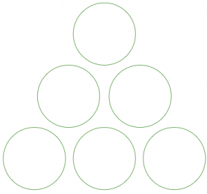
Place the digits 1, 2, 3, 4, 5, 6 in the circles so that the sum on each side of the triangle is 12. Each circle gets one digit, and each digit is used exactly once.
- Answer
-
To solve this puzzle, we need to place the digits 1, 2, 3, 4, 5, and 6 in the circles so that the sum along each side of the triangle equals 12. Here is a possible arrangement. Top = 5, Middle Left = 1, Bottom Left = 6, Middle Right = 3, Bottom Right = 4, Bottom Middle = 2.
As pictured in the table below, the hexagon train made with 1 hexagon has a perimeter of 6; the hexagon train made with 2 hexagons has a perimeter of 10; and the hexagon train made with 3 hexagons has a perimeter of 14. What is the perimeter of the hexagon train made with 4 hexagons? 5 hexagons? 100 hexagons?

- Answer
-
Each additional hexagon increases the perimeter by 4, as two sides overlap with the previous hexagon. The pattern follows the rule: Perimeter = 4 (figure number) + 2 .
4 Hexagons: P = 4(4) + 2 = 18
5 Hexagons: P = 5(4) + 2 = 22
100 Hexagons: P = 100(4) + 2 = 402