

3.2: Developing Multiplicative and Divisional Thinking
- Page ID
- 181694
\( \newcommand{\vecs}[1]{\overset { \scriptstyle \rightharpoonup} {\mathbf{#1}} } \)
\( \newcommand{\vecd}[1]{\overset{-\!-\!\rightharpoonup}{\vphantom{a}\smash {#1}}} \)
\( \newcommand{\dsum}{\displaystyle\sum\limits} \)
\( \newcommand{\dint}{\displaystyle\int\limits} \)
\( \newcommand{\dlim}{\displaystyle\lim\limits} \)
\( \newcommand{\id}{\mathrm{id}}\) \( \newcommand{\Span}{\mathrm{span}}\)
( \newcommand{\kernel}{\mathrm{null}\,}\) \( \newcommand{\range}{\mathrm{range}\,}\)
\( \newcommand{\RealPart}{\mathrm{Re}}\) \( \newcommand{\ImaginaryPart}{\mathrm{Im}}\)
\( \newcommand{\Argument}{\mathrm{Arg}}\) \( \newcommand{\norm}[1]{\| #1 \|}\)
\( \newcommand{\inner}[2]{\langle #1, #2 \rangle}\)
\( \newcommand{\Span}{\mathrm{span}}\)
\( \newcommand{\id}{\mathrm{id}}\)
\( \newcommand{\Span}{\mathrm{span}}\)
\( \newcommand{\kernel}{\mathrm{null}\,}\)
\( \newcommand{\range}{\mathrm{range}\,}\)
\( \newcommand{\RealPart}{\mathrm{Re}}\)
\( \newcommand{\ImaginaryPart}{\mathrm{Im}}\)
\( \newcommand{\Argument}{\mathrm{Arg}}\)
\( \newcommand{\norm}[1]{\| #1 \|}\)
\( \newcommand{\inner}[2]{\langle #1, #2 \rangle}\)
\( \newcommand{\Span}{\mathrm{span}}\) \( \newcommand{\AA}{\unicode[.8,0]{x212B}}\)
\( \newcommand{\vectorA}[1]{\vec{#1}} % arrow\)
\( \newcommand{\vectorAt}[1]{\vec{\text{#1}}} % arrow\)
\( \newcommand{\vectorB}[1]{\overset { \scriptstyle \rightharpoonup} {\mathbf{#1}} } \)
\( \newcommand{\vectorC}[1]{\textbf{#1}} \)
\( \newcommand{\vectorD}[1]{\overrightarrow{#1}} \)
\( \newcommand{\vectorDt}[1]{\overrightarrow{\text{#1}}} \)
\( \newcommand{\vectE}[1]{\overset{-\!-\!\rightharpoonup}{\vphantom{a}\smash{\mathbf {#1}}}} \)
\( \newcommand{\vecs}[1]{\overset { \scriptstyle \rightharpoonup} {\mathbf{#1}} } \)
\(\newcommand{\longvect}{\overrightarrow}\)
\( \newcommand{\vecd}[1]{\overset{-\!-\!\rightharpoonup}{\vphantom{a}\smash {#1}}} \)
\(\newcommand{\ket}[1]{\left| #1 \right>}\)
\(\newcommand{\bra}[1]{\left< #1 \right|}\)
\(\newcommand{\braket}[2]{\left< #1 \vphantom{#2} \right| \left. #2 \vphantom{#1} \right>}\)
\(\newcommand{\braopket}[3]{\left< #1 \vphantom{#2}\vphantom{#3} \right| #2 \vphantom{#1}\vphantom{#3} \left| #3 \vphantom{#1}\vphantom{#2} \right>}\)
\(\newcommand{\qmvec}[1]{\mathbf{\vec{#1}}}\)
\(\newcommand{\op}[1]{\hat{\mathbf{#1}}}\)
\(\newcommand{\expect}[1]{\langle #1 \rangle}\)
\(\newcommand{\dfn}[1]{\emph{\textbf{#1}}}\)
Children develop multiplication and division understanding through informal strategies before mastering formal procedures. Initially, they rely on repeated addition, tally marks, or halving strategies to make sense of multiplication, while division often begins with fair-sharing or repeated subtraction (Feike, Schwingendorf, and Gregg, 2018). As they build number sense, place value understanding, and fluency in addition, they transition from additive to multiplicative thinking—a crucial milestone in mathematical reasoning (NCTM, 2020). Encouraging children to explore and construct their own problem-solving strategies fosters deeper comprehension, rather than rote memorization of algorithms. Through hands-on experiences, mental math strategies, and recognizing mathematical properties like commutativity, associativity, and distributivity, children develop a rich, conceptual understanding of multiplication and division that supports their long-term mathematical success (Feike, Schwingendorf, and Gregg, 2018).
Multiplication
More Math Moments of Brilliance - What is Nathan Thinking?
Task 1: Think about and then discuss with peers how you think a young child could solve the problem 6 x 5.
Task 2: Watch the short video of Nathan calculating 6 x 5.
Task 3: WOW! What did he do? Why does it work? Think and About and discuss with peers.
Task 4: Does his process always work? Come up with examples and/or counter examples.
🧠Let's Listen to Learn❤️
We use three models to discuss multiplication: the repeated addition model, the rectangular array model, and the Cartesian-product model. Also, we investigate the properties of multiplication.
If a and b are whole numbers, then a \(\times\) b = b + b+ b+ b + ... + b, where there are a addends of b in this sum.
I like to think of using the definition like this:
3 \(\times\) 4 means 3 fours added together or 3 \(\times\) 4 = 4 + 4 + 4 = 12
4 \(\times\) 3 means 4 threes added together, or 4 \(\times\) 3 = 3 + 3 + 3 + 3 = 12
5 \(\times\) 2 means 5 twos added together, or 5 \(\times\) 2 = 2 + 2 + 2 + 2 + 2 = 10
2 \(\times\) 5 means 2 fives added together, or 2 \(\times\) 5 = 5 + 5 = 10
Note that although 3 \(\times\) 4 gives the same answer as 4 \(\times\) 3, it does not mean the same thing! One means 4 + 4 + 4 and the other means 3 + 3 + 3 + 3.
These problems can be modeled using the set model and the measurement model. These models look similar to the ones that we used for addition, since we are merely adding repeatedly. Figure 3.2.1

Figure \(\PageIndex{1}\)
Before we delve any further into this discussion, I want you to use the repeated addition definition to compute the following:
Use the repeated addition definition of multiplication to compute the following. First, write out the meaning of the multiplication, and then compute the answer.
a. 6 \(\times\) 3 =
b. 2 \(\times\) 9 =
c. 9 \(\times\) 2 =
- Answer
-
a) 3 + 3 + 3 + 3 + 3 + 3 = 18
b) 9 + 9 = 18
c) 2 + 2 + 2 + 2 + 2 + 2 + 2 + 2 + 2 = 18
Now, it may seem obvious to you that 3 \(\times\) 4 is the same answer as 4 \(\times\) 3. That's because you've no doubt been using the commutative property of addition for years. Whether or not you really thought about why it was true is another thing. But, although 3 \(\times\) 4 gives the same answer as 4 \(\times\) 3, it does not mean the same thing. One means 4 + 4 + 4 and the other means 3 + 3 + 3 + 3. To a child just learning about addition and multiplication, there is no reason for them to conclude that one sum (4 + 4 + 4) happens to give the same answer as the other sum (3 + 3 + 3 + 3). For instance, if I was asked to compute the following two sums, it wouldn't be evident to me at all that the answer to each would be end up being the same:
| 17 + 17 + 17 + 17 and 4 + 4 + 4 + 4 + 4 + 4 + 4 + 4 + 4 + 4 + 4 + 4 + 4 + 4 + 4 + 4 + 4 |
Actually, I find it quite amazing that they are equal. But, indeed they are, because the first sum comes from the multiplication problem 4 \(\times\) 17 (since there are 4 seventeens added together), and the second sum comes from the multiplication problem 17 \(\times\) 4 (since there are 17 fours added together). Later, when we discuss a more geometrical definition for multiplication, it becomes obvious why the commutative property of multiplication is true.
The commutative property of multiplication for whole numbers states that if a and b are any two numbers, then
\[a \times b = b \times a. \nonumber \]
Remember that the commutative property means there has been an order change. To verify the commutative property of multiplication, you need to use the repeated addition definition of multiplication and add from left to right, one number at a time. The next example shows how to verify the commutative property of multiplication, given a set of two numbers.
The associative property of multiplication states that if a, b and c are any three numbers, then \((a \times b) \times c = a \times (b \times c\)).
Before going on to any more properties, we'll practice verifying that the associative property of multiplication is true for some numbers in base ten later on, we'll do it in other bases, too. The associative property requires three numbers (they don't have to be three different numbers) and there are different expressions on each side of the equation. The difference between the left and right sides is that the parentheses are around a different pair of numbers. Remember that the associative property means there is a parentheses change, whereas the commutative property means there has been an order change. To verify, you need to use the order of operations when simplifying each side. If each expression simplifies to same thing, the equation is true. In the order of operations, you always simplify what is in parentheses first. The following are some examples of how to verify the associative property of multiplication, given a set of three numbers.
Verify the associative property of multiplication is true using the three numbers {4, 5, 7} in your example.
- Answer
-
Note: Since the associative property states \((a \times b) \times c = a \times (b \times c)\), one of the numbers given is put in for a, the other for b and the other for c. The choice is yours. For example, we can show any of the following six equations are true:
a. \((4 \times 5) \times 7 = 4 \times (5 \times 7)\) or d. \((4 \times 7) \times 5 = 4 \times (7 \times 5)\) b. \((5 \times 4) \times 7 = 5 \times (4 \times 7)\) or e. \((7 \times 4) \times 5 = 7 \times (4 \times 5)\) c. \((7 \times 5) \times 4 = 7 \times (5 \times 4)\) or f. \((5 \times 7) \times 4 = 5 \times (7 \times 4)\).
The distributive property of multiplication over addition for whole numbers states that if a, b and c are any three numbers, then \(a \times (b + c) = (a \times b) + (a \times c)\).
Note: \(a \times (b - c) = (a \times b) - (a \times c)\), when \(b\ge c\).
The distributive property makes more complex multiplications more manageable by leveraging simpler, known multiplication facts. That visual breakdown bridges symbolic understanding and physical representation, helping the math "stick." You can see why the property makes sense.
Now, it's time to practice verifying the distributive property of multiplication over addition is true for some numbers in base ten — later on, we'll do it in other bases, too. The distributive property requires three numbers (they don't have to be three different numbers) and there are two sides of an equation to verify. Note the difference between the left and right sides. To verify, you need to use the order of operations when simplifying each side. In the order of operations, you always simplify what is in parentheses first. If each expression simplifies to same thing, the equation is true. The following are some examples of how to verify the distributive property of multiplication, given a set of three numbers.
Verify the distributive property of multiplication is true using the three numbers {4, 5, 7} in your example.
- Answer
-
Note: Since the distributive property states \(a \times (b + c) = (a \times b) + (a \times c)\), one of the numbers given is put in for a, the other for b and the other for c. The choice is yours. For example, we can show any of the following six equations are true:
a. \(4 \times (5 + 7) = (4 \times 5) + (4 \times 7)\) or d. \(5 \times (7 + 4) = (5 \times 7) + (5 \times 4)\) b. \(4 \times (7 + 5) = (4 \times 7) + (4 \times 5)\) or e. \(7 \times (4 + 5) = (7 \times 4) + (7 \times 5)\) c. \(5 \times (4 + 7) = (5 \times 4) + (5 \times 7)\) or f. \(7 \times (5 + 4) = (7 \times 5) + (7 \times 4)\)
Wonder, Play, Grow
Compute the following products using thinking strategies.
a) 2 x 34 b) 5(37 x 2) c) 7(25)
The number 1 is the unique whole number such that for every whole number a,
\(a \times 1 = (1 \times a) =a\).
The product of two whole numbers is a whole number.
When two odd whole numbers are multiplied together, the product is odd; thus the set of odd numbers is closed under multiplication. Closure is a useful idea, since if we are multiplying two (or more) odd numbers and the product we calculate is even,we can conclude that our product is incorrect. The set {2, 5, 8,11,14, . . . } is not closed under multiplication, since 2 ¥ 5 = 10 and 10 is not in the set.
For every whole number, a,
a x 0 = 0 x a = 0.
There is another way to define multiplication using Set Theory. In order to do this, we have to remember how to take the Cartesian product of two sets, A and B.
The Cartesian product of set A with set B, which is written \(A \times B\) and is read as "A cross B" is the set of all possible ordered pairs (a,b), where a ∈ A and b ∈ B.
If you are finding the Cartesian product, the answer is a set that contains ordered pairs. Using set builder notation, we can write 𝐴×𝐵={(a,b) | a∈𝐴 and b∈𝐵}.
a) If A = {x, y, z} and B = {a, b}, find \(A \times B\).
b) If E = {1, 2} and F = {2, 3}, find \(E \times F\).
- Answer
-
a) \(A \times B\) = {(x, a), (x, b), (y, a), (y, b), (z, a), (z, b)}
b) \(E \times F\) = {(1, 2), (1, 3), (2, 2), (2, 3)}
Notice that when finding a Cartesian product, all possible pairs are formed where the first element comes from the first and the second element comes from the second set. Also observe that in Example 3.2.4 (a), there are three elements in the first set, two in the second, and six in their Cartesian product, and that 3 x 2 = 6. Similarly, in (b), these sets can be used to find the whole-number product 2 x 2 = 4.
For completion, it is good to know the Set Theory Definition for Multiplying. For any two sets A and B, \(\bf n(A) \cdot n(B) = n(A \times B)\). Note: There are no restrictions on what elements you choose for sets A and B. They can be disjoint or they can have elements in common. It’s up to you.
Here's a more geometrical approach to defining multiplication of two whole numbers.
To find the product of any two whole numbers, m and n, make a rectangular array of objects having m rows and n columns. The product of m and n, written \(m \times n\), equals the number of objects in the array.
The cool thing about using this geometrical approach is that any objects can be used, and one only needs to be able to count to get the answer. You don't need to use addition in order to multiply! I personally advocate having lots of graph paper around for anyone just learning to multiply. To compute \(4 \times 7\), you or the learner can mark off a rectangle on the graph paper that has 4 rows and 7 columns of boxes. The number of boxes in the rectangle is the answer to the problem. This is a useful tool for first learning a particular multiplication fact, or for anyone (adults, too) who forgot a fact and needs to figure it out again. The "objects" used on a graph paper are the individual boxes on the graph paper.
Here is how six different students might geometrically show how to multiply \(4 \times 7\).
 |
 |
 |
 |
 |
 |
There is no point to making anyone stress out if they forgot, didn't memorize or couldn't recall the answer to \(4 \times 7\). The point is to KNOW WHAT MULTIPLICATION MEANS so you can figure a problem out again if you have to. Of course, there is merit to using flashcards and eventually memorizing basic multiplication facts like your multiplication tables. If not, it takes longer to do problems, you aren't able to focus on more advanced issues, and you might not trust your own mind. You shouldn't have to think about multiplication every time you have to multiply two numbers together, but you should be able to think about it. Knowing how to get the answer is better than having memorized a bunch of facts if you don't know where they came from, what multiplication really means, or how to figure it out again in case you forget the answer to some fact. And, as far as I'm concerned, nothing's wrong with using your fingers, either! Let people do what is comfortable for them, if they understand and can get the right answer, that's GREAT!
Write the multiplication problem represented by each geometrical representation:
|
a. ____  |
b. ____  |
|
c. ____  |
d. ____  |
- Answer
-
a) 5 x 5 (number of objects) b) 3 x 10 (number of objects) c) 4 x 14 (number of squares) d) 3 x 7 (number of squares)
Wonder, Play, Grow
Task 1: Without using paper and the traditional way to multiply, find 18 x 5. (the answer is 90).
Task 2: View the video (maybe twice).
Task 3: Write down at least two ways you heard students solve the problem.Task 4: Make up a multiplication problem and solve it using thinking strategies. Share with a peer.
Division
Young children, especially those who do not yet have fluency with division facts or an understanding of multiplication as the inverse of division, solve division problems using two distinct strategies: Partitioning Model (Fair Sharing) and Measurement Model (Repeated Subtraction). These two approaches correspond to the two major conceptual models of division. Consider \(18 \div 3 = 6\).
Partitioning (Fair Sharing Model)Partitioning division involves dividing a total quantity into a specified number of equal groups and determining how many objects are in each group. This model is often more intuitive for young children since it aligns with real-life experiences of sharing equally. Fair Sharing Example Problem: "If you have 18 cookies and want to divide the cookies up equally amongst your three children, how many cookies should you give to each child?" How a Child Might Solve It:
Key Characteristics of Partitioning Division:
|
Measurement Model (Repeated Subtraction)Repeated subtraction division involves forming groups of a fixed size and determining how many such groups can be made. This model is sometimes called the measurement model because it mimics the process of measuring a length using repeated units. Measurement Division Example Problem: "If you have 18 cookies and want to make baggies having three cookies in each to put in lunch boxes, how many baggies will you be able to make?" How a Child Might Solve It:
Alternatively, a child might solve it using subtraction:
Key Characteristics of Measurement Division:
|


Partitioning into (Equal) Subsets (Fair Share Model)
In this interpretation, the divisor is the number of subsets in which to disburse something. The dividend, 18, must be divided amongst 3 equal subsets (3 is the divisor). The quotient (answer to the division problem) will be the number of elements (6) placed in each subset (the kids, in this case.) The task is to partition 18 cookies into 3 equal subsets.
Repeated Subtraction (Measurement Model)
In this interpretation, the divisor is the number of elements that will go into each subset. Each time the divisor (3) is subtracted from the dividend (18), a subset is formed. After all elements have been disbursed, the quotient (answer) is found by counting how many subsets were formed.
Word Problems requiring division generally fall into the category of Repeated Subtraction or Partitioning into Subsets. After reading a word problem, you should be able to analyze and interpret it as a problem that requires Partitioning into Subsets or Measurement / Repeated Subtraction to solve the problem, and then be able to draw a picture using that interpretation. Also, for any division problem given, you should be able to write two distinct word problems, one for each interpretation, and draw a picture for each interpretation, and be able to explain and show all the steps necessary to solve the problem.
🧠Let's Listen to Learn❤️
Understanding these two fundamental models of division, future teachers can help young learners develop a solid mathematical foundation and flexible problem-solving skills.
1) Work with your peers to identify whether the following problems are using measurement (MD) or partitive division (PD) (if in doubt, try drawing a picture to represent the situation.
a) Jim tied 30 sticks into 3 equal bundles. How many sticks were in each bundle?
b) 24 balls are packed into boxes of 6. How many boxes are there?
c) Mr. Lin tied 195 books into bundles of 5 each. How many bundles were there?
d) 6 children shared 84 balloons equally. How many balloons did each child get?
2) Work with peers to make up a word problem for the following using the procedure: (Be prepared to share with the class)
a) measurement division for 84 ÷ 21.
b) partitive division for 90 ÷ 5.
Division is the operation that undoes multiplication. Students can rely on this fact to learn basic division facts. For instance, since 6 \(\cdot\) 7 = 42, then \(42 \div 6 = 7\) and \(42 \div 7 = 6\). Below is a formal definition of division.
If a and b are any whole numbers, a \(\div\) b is defined to be the unique number, c, under the following conditions: \(a \div b = c\) if and only if a = b \(\cdot\) c. If there is no number, c, that exists, or if there is more than one unique number that can be put in for c, then \(a \div b\) is said to be undefined.
The symbol a \(\div\) b is read “a divided by b.” Also, a is called the dividend, b is called the divisor, and c is called the quotient or missing factor.
Use the missing-factor approach of division to find the answer to \(\bf 21 \div 3\).
First, note that \(21 \div 3\) = ____ means 21 = 3 \(\cdot\) _____ Second, try to fill in the blank in the multiplication problem with a unique number to make the equation, 21 = 3 \(\cdot\) _____, true: 21 = 3 \(\cdot \underline{7}\). If the number filled in is the only possible solution (unique), then that is the answer to the division problem. Therefore, \(21 \div 3\) = \(\underline{7}\). You do not need to write this paragraph for your solution. Below is how to write the solution.
- Answer
-
Since \(21 = 3 \cdot \underline{7}\), then \( 21 \div 3 = \underline{7}\).
Use the missing-factor approach of division to find the following quotients:
| a. \(0 \div 13\) |
| b. \(12 \div 1\) |
| c. \(X \div 1\) (Assume X is any number.) |
| d. \(0 \div Y\) (Assume Y is any nonzero number.) |
- Answer
-
a) \(0\div 13\) = 0 since 0 = 13 x 0
b) \(12 \div 1\) = 12 since 12 = 12 x 1
c) \(X \div 1\) = X since X = X x 1
d) \(0\div Y\) = 0 since 0 = Y x 0
Example 7c illustrates that any number divided by 1 is itself. In other words, \(\bf a \div 1 = a\) for all values of a.
Example 7d illustrates that zero divided by any nonzero whole number is 0. In other words, \(\bf 0 \div a = 0\), for all nonzero values of a.
Let's explore what happens when we divided by zero.
Discuss with your peers how to use the missing-factor approach to figure out the following quotients \(8 \div 0\) and \(0 \div 0\).
Once you have a chance to give and take ideas, take a look at an explanation.
- Explanation
-
There is no number that will make the equation, 8 = 0 \(\cdot\) ____ true, since any number put in the blank will make the right hand side of the equation zero, which can never equal the left-hand side of the equation, which is 8. Therefore, \( 8 \div 0\) is not defined.
There is no unique number that can be put in the blank to make the equation 0 = 0 \(\cdot\) ____ true, since any number will make it true. Therefore, \(0 \div 0\) is called indeterminate.
Division by 0 is undefined
To prove that division by zero is undefined, two cases must be shown. Below is a complete proof to show that division by zero is undefined.
Problem: Prove that division by zero is undefined
Solution: The goal is to show that \(a \div 0\) is undefined for all values of a. There are two cases to consider Case 1: \(a \neq 0\); Case 2: a = 0.
Case 1: Let \(a \neq 0\). There is no unique number that could be put in the blank to make the equation, a = 0 \(\cdot\) ____, true because the left-hand side of the equation is not zero (since \(a \neq 0\)), and any number put in the blank will make the right hand side of the equation zero. Therefore, when \(a \neq 0\), \(a \div 0\) is not defined.
Case 2: Let a = 0. There is no unique number that can be put in the blank to make the equation 0 = 0 \(\cdot\) ____ true, since any number will make it true. Therefore, \(0 \div 0\) is indeterminate.
It takes practice writing this proof. You'll need to practice writing it several times to master the problem. One option is to memorize the proof shown above by writing it out a few times until you really get the idea. This would make a good exam question.
If a and b are any whole numbers with b ≠ 0, then there exist unique whole numbers q and r such that a = bq + r, where 0 ≤ r < b.
Here b is called the divisor, q is called the quotient, and r is the remainder. Notice that the remainder is always less than the divisor. Also, when the remainder is 0, this result coincides with the usual dei nition of whole-number division.
Find the quotient and remainder for 25 \(\div \) 7.
- Answer
-
7 x 3 = 21, so 25 = 7 x 3 + 4, The quotient is 3 and the remainder is 4.
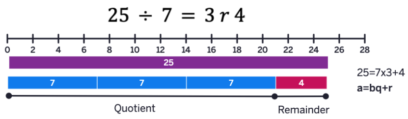
The example above can also be represented using repeated subtraction. In general, to find a ÷ b using the repeated-subtraction approach, subtract b successively from a and from the resulting differences until a remainder r is reached, where r < b. The number of times b is subtracted is the quotient q. Figure 3.2.2.

Figure 3.2.3 visually illustrates the key relationships among the four basic whole-number operations. It shows how multiplication builds on repeated addition, subtraction is understood through the missing-addend approach, and other operations connect similarly. A crucial takeaway from this diagram is that a strong grasp of addition forms the foundation for success in subtraction, multiplication, and division.

Future Teacher Thinking: Understanding the Progression of Multiplication and Division
Mathematics instruction in multiplication and division is most effective when it unfolds over time, allowing students to move through a developmental progression. The YouTube videos by Graham Fletcher on the "Progression of Multiplication" and "Progression of Division" demonstrate how students benefit from beginning with concrete representations, then moving to pictorial models, and eventually to abstract notation. This is known as the Concrete-Pictorial-Abstract (CPA) approach.
Take a look at the videos and discuss with your peers about what is still circling in your head, what really resonated with you, and what is one thing you do not want to forget.
|
Progression of Multiplication |
Progression of Division |
Key Concepts:
- Concrete to Abstract Learning (CPA): Students begin with hands-on experiences (like manipulatives and drawings), which ground their understanding before moving into symbolic representations and algorithms.
- Models in Division: Two key conceptual models are used—measurement (repeated subtraction) and fair share. These models help students understand the meaning of division in different contexts.
- Multiplication and Division Representations: Arrays, area models, and base-10 blocks help bridge the gap between understanding operations and executing them efficiently.
- From Inefficient to Efficient: While drawing objects or subtracting repeatedly may seem slow, these methods build the foundation for flexible strategies like partial products and partial quotients.
- Inverse Relationship: The two operations are closely connected. Arrays and area models visually demonstrate how multiplication and division are inverse operations.
- Distributive Property: This property becomes clearer to students when represented with area models or base-10 blocks, making sense of abstract equations.
- Standard Algorithms: Rather than being introduced first, standard algorithms are shown later—once students understand why the steps work.
- Teacher’s Role: Educators are encouraged to let the context drive the mathematics, enabling students to make sense of problems and explore solutions before being taught procedures