16.5: Surfaces and Area
- Page ID
- 2639
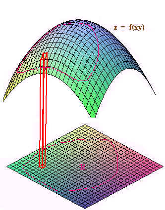
In first year calculus we have seen how to find the surface area of revolution. Now that we have the power of double integration, we are ready to take on the surface area for more general surfaces. We can think of a smooth surface as a quilt flapping in the wind. It consists of many rectangles patched together. More generally and more accurately, let \(z = f(x,y)\) be a surface in \(\mathbb{R}^3\) defined over a region \(R\) in the \(xy\)-plane. Cut the \(xy\)-plane into rectangles. Each rectangle will project vertically to a piece of the surface as shown in the figure below. Although the area of the rectangle in \(R\) is
\[\text{Area} = \Delta y\,\Delta x\nonumber \]

The area of the corresponding piece of the surface will not be \(\Delta y\, \Delta x\) since it is not a rectangle. Even if we cut finely, we will still not produce a rectangle, but rather will approximately produce a parallelogram. With a little geometry we can see that the two adjacent sides of the parallelogram are (in vector form)
\[ \vec{u} = \Delta x \hat{\textbf{i}} + f_x(x,y)\Delta x \hat{\textbf{k}}\nonumber \]
and
\[ \vec{v} = f_y(x,y) \Delta y \hat{\textbf{i}} + \Delta{y} \hat{\textbf{k}}\nonumber \]
We can see this by realizing that the partial derivatives are the slopes in each direction. If we run \( \Delta x\) in the \(\hat{\textbf{i}}\) direction, then we will rise \( f_x(x,y) \Delta x\) in the \(\hat{\textbf{k}}\) direction so that
\[ \text{rise/run} = f_x(x,y) \nonumber \]
which agrees with the slope idea of the partial derivative. A similar argument will confirm the equation for the vector \(\text{v}\). Now that we know the adjacent vectors we recall that the area of a parallelogram is the magnitude of the cross product of the two adjacent vectors. We have
\[\begin{align*}|v \times w| &= \begin{vmatrix} \hat{\textbf{i}} &\hat{\textbf{j}} & \hat{\textbf{k}} \\[4pt] \Delta x & 0 & f_x(x,y) \\ 0 & \Delta y & f_y (x,y)\Delta y \end{vmatrix} \\[4pt] &= | -(f_y (x,y)\Delta y\Delta x) \hat{\textbf{i}} - (f_x (x,y) \Delta y \Delta x) \hat{\textbf{j}} + (\Delta y \Delta x) \hat{\textbf{k}} | \\[4pt] &= \sqrt{f_y^2 (x,y) (\Delta y \Delta x)^2 + f_x^2 (x,y) (\Delta y \Delta x)^2 +(\Delta y \Delta x)^2 } \\[4pt] &= \sqrt{f_y^2 (x,y) + f_x^2 (x,y) +1 } \; \Delta y \Delta x. \end{align*}\nonumber \]
This is the area of one of the patches of the quilt. To find the total area of the surface, we add up all the areas and take the limit as the rectangle size approaches zero. This results in a double Riemann sum, that is a double integral. We state the definition below.
Definition: Surface Area
Let \(z = f(x,y)\) be a differentiable surface defined over a region \(R\). Then its surface area is given by
\[ \text{Surface Area} = \iint_R \sqrt{1 + f_x^2(x,y) + f_y^2(x,y) }\; dy\, dx.\nonumber \]
Example \(\PageIndex{1}\)
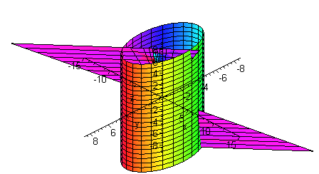
Find the surface area of the part of the plane
\[ z = 8x + 4y\nonumber \]
that lies inside the cylinder
\[ x^2 + y^2 = 16.\nonumber \]

Solution
We calculate partial derivatives
\[ f_x(x,y) = 8 \nonumber \]
and
\[ f_y(x,y) = 4 \nonumber \]
so that
\[ 1 + f_x^2(x,y) + f_y^2(x,y) = 1 + 64 + 16 = 81. \nonumber \]
Taking a square root and integrating, we get
\[ \iint 9 \, dy\,dx. \nonumber \]
We could work this integral out, but there is a much easier way. The integral of a constant is just the constant times the area of the region. Since the region is a circle, we get
\[ \text{Surface Area} = 9(16\pi) = 144\pi .\nonumber \]
In reality, since there is a square root in the formula, most surface area calculations require intensive integration skills or the use of a computer. The prior example and the next example are not meant to deceive, but rather to show how the essence of surface area problems work without the integration difficulty clouding your understanding.
Example \(\PageIndex{2}\)
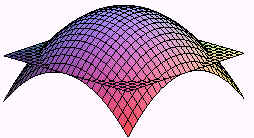
Find the surface area of the part of the paraboloid
\[ z = 25 - x^2 - y^2 \nonumber \nonumber \]
that lies above the xy-plane.

Solution
We calculate partial derivatives
\( f_x(x,y) = -2x \) and \(f_y(x,y) = -2y \)
so that
\[ 1 + f_x^2(x,y) + f_y^2(x,y) = 1 + 4x^2 + 4y^2. \nonumber\nonumber \]
At this point if we listen closely, we should hear a little voice pleading "Polar Coordinates". We listen to its call and realize that the region is just the circle with \( r = 5\).
Now convert the integrand to polar coordinates to get
\[ \int_0^{2\pi}\int_o^5 \sqrt{1+4r^2} \; r \, dr\, d\theta . \nonumber\nonumber \]
Now let
\[ u = 1 + 4r^2 \nonumber\nonumber \]
and
\[du = 8r\,dr \nonumber\nonumber \]
and substitute
\[\dfrac{1}{8}\int_0^{2\pi} \int_0^{101} u^{1/2}du\,d\theta = \left. \dfrac{1}{12} \int_0^{2\pi} u^{2/3} \right|_0^{101} \approx 530.95. \nonumber\nonumber \]
Surface Area Differentials for Parametrized Surface
\[d\sigma = |\mathbf{r}_u\times\mathbf{r}_v|dudv \nonumber \]
Surface Area Differential
\[\int \int _sd\sigma\nonumber \]
Differential formula for Surface Area
- Larry Green (Lake Tahoe Community College)
Integrated by Justin Marshall.


