5.3: Cauchy’s Form of the Remainder

Learning Objectives

• Explain Cauchy's form of the remainder

In his 1823 work, Résumé des le¸cons données à l’ecole royale polytechnique sur le calcul infintésimal, Augustin Cauchy provided another form of the remainder for Taylor series.

Theorem \(\PageIndex{1}\): Cauchy’s Form of the Remainder

Suppose \(f\) is a function such that \(f^{(n+1)}(t)\) is continuous on an interval containing \(a\) and \(x\). Then

\[f(x) - \left ( \sum_{j=0}^{n}\dfrac{f^{(j)}(a)}{j!}(x-a)^j \right ) = \dfrac{f^{(n+1)}(c)}{n!}(x-c)^n(x-a)\]

where \(c\) is some number between \(a\) and \(x\).

Exercise \(\PageIndex{1}\)

Prove Theorem \(\PageIndex{1}\) using an argument similar to the one used in the proof of Theorem 5.2.1. Don’t forget there are two cases to consider.

Using Cauchy’s form of the remainder, we can prove that the binomial series

\[1 + \dfrac{1}{2}x + \dfrac{\dfrac{1}{2}\left ( \dfrac{1}{2} -1 \right )}{2!}x^2 + \dfrac{\dfrac{1}{2}\left ( \dfrac{1}{2} -1 \right )\left ( \dfrac{1}{2} -2 \right )}{3!}x^3 + \cdots\]

converges to \(\sqrt{1+x}\) for \(x ∈ (-1,0)\). With this in mind, let \(x\) be a fixed number with \(-1 < x < 0\) and consider that the binomial series is the Maclaurin series for the function \(f(x) = (1 + x)^\dfrac{1}{2}\). As we saw before,

\[f^{(n+1)}(t) = \left ( \dfrac{1}{2} \right )\left ( \dfrac{1}{2} -1 \right )\cdots \left ( \dfrac{1}{2} -n \right )(1+t)^{\dfrac{1}{2} - (n+1)}\]

so the Cauchy form of the remainder is given by

\[0 \leq \left | \dfrac{f^{(n+1)}(c)}{n!}(x-c)^n(x-0) \right | = \left | \dfrac{\dfrac{1}{2}\left ( \dfrac{1}{2} -1 \right )\cdots \left ( \dfrac{1}{2} -n \right )}{n!} \dfrac{(x-c)^n}{(1+c)^{n+\dfrac{1}{2}}}\cdot x\right |\]

where \(c\) is some number with \(x ≤ c ≤ 0\). Thus we have

\[\begin{align*} 0 &\leq \left | \dfrac{\left ( \dfrac{1}{2} \right )\left ( \dfrac{1}{2} -1 \right )\cdots \left ( \dfrac{1}{2} -n \right )}{n!} \dfrac{(x-c)^n x}{(1+c)^{n + \dfrac{1}{2}}} \right | \\ &= \dfrac{\left ( \dfrac{1}{2} \right )\left ( 1 -\dfrac{1}{2} \right )\cdots \left ( n - \dfrac{1}{2} \right )}{n!} \dfrac{\left |x-c \right |^n\left | x \right |}{(1+c)^{n + \dfrac{1}{2}}}\\ &= \dfrac{\left ( \dfrac{1}{2} \right )\left ( \dfrac{1}{2} \right )\left ( \dfrac{3}{2} \right )\left ( \dfrac{5}{2} \right )\cdots \left ( \dfrac{2n-1}{2} \right )}{n!})\dfrac{(c-x)^n}{(1+c)^n}\dfrac{\left |x \right |}{\sqrt{1+c}}\\ &\leq \dfrac{1\cdot 1\cdot 3\cdot 5\cdots (2n-1)}{2^{n+1}n!} \left (\dfrac{c-x}{1+c} \right )^n\dfrac{\left |x \right |}{\sqrt{1+c}}\\ &= \dfrac{1\cdot 1\cdot 3\cdot 5\cdot (2n-1)}{2\cdot 2\cdot 4\cdot 6\cdots 2n} \left (\dfrac{c-x}{1+c} \right )^n\dfrac{\left |x \right |}{\sqrt{1+c}}\\ &= \dfrac{1}{2} \cdot \dfrac{1}{2} \cdot \dfrac{3}{4} \cdot \dfrac{5}{6} \cdots \dfrac{2n-1}{2n}\cdot \left (\dfrac{c-x}{1+c} \right )^n\dfrac{\left |x \right |}{\sqrt{1+c}}\\ &\leq \left (\dfrac{c-x}{1+c} \right )^n\dfrac{\left |x \right |}{\sqrt{1+c}} \end{align*}\]

Notice that if \(-1 < x ≤ c\), then \(0 < 1 + x ≤ 1 + c\). Thus \(0 < \dfrac{1}{1+c} \leq \dfrac{1}{1+x}\) and \(\dfrac{1}{\sqrt{1+c}} \leq \dfrac{1}{\sqrt{1+x}}\). Thus we have

\[0 \leq \left |\dfrac{\left ( \dfrac{1}{2} \right )\left ( \dfrac{1}{2} -1 \right )\cdots \left ( \dfrac{1}{2} -n \right )}{n!} \dfrac{(x-c)^n x}{(1+c)^{n + \dfrac{1}{2}}} \right | \leq \left (\dfrac{c-x}{1+c} \right )^n\dfrac{\left |x \right |}{\sqrt{1+c}}\]

Exercise \(\PageIndex{2}\)

Suppose \(-1 < x ≤ c ≤ 0\) and consider the function \(g(c) = \dfrac{c-x}{1+x}\). Show that on \([x,0]\), \(g\) is increasing and use this to conclude that for \(-1 < x ≤ c ≤ 0\),

\[\dfrac{c-x}{1+x} \leq \left | x \right | \nonumber\]

Use this fact to finish the proof that the binomial series converges to \(\sqrt{1+x}\) for \(-1 < x < 0\).

The proofs of both the Lagrange form and the Cauchy form of the remainder for Taylor series made use of two crucial facts about continuous functions.

First, we assumed the Extreme Value Theorem: Any continuous function on a closed bounded interval assumes its maximum and minimum somewhere on the interval.

Second, we assumed that any continuous function satisfied the Intermediate Value Theorem: If a continuous function takes on two different values, then it must take on any value between those two values.

Figure \(\PageIndex{1}\): Augustin Cauchy

Mathematicians in the late 1700’s and early 1800’s typically considered these facts to be intuitively obvious. This was natural since our understanding of continuity at that time was, solely, intuitive. Intuition is a useful tool, but as we have seen before it is also unreliable. For example consider the following function.

\[f(x) = \begin{cases} x\sin \left (\dfrac{1}{x} \right ) & \text{ if } x \neq 0 \\ 0 & \text{ if } x= 0 \end{cases}\]

Is this function continuous at \(0\)? Near zero its graph looks like this:

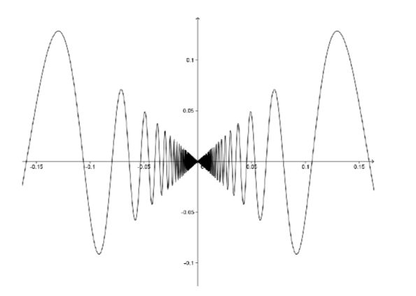
Figure \(\PageIndex{2}\): Graph of the function above.

but this graph must be taken with a grain of salt as \(\sin \left (\dfrac{1}{x} \right )\) oscillates infinitely often as \(x\) nears zero. No matter what your guess may be, it is clear that it is hard to analyze such a function armed with only an intuitive notion of continuity. We will revisit this example in the next chapter.

As with convergence, continuity is more subtle than it first appears. We put convergence on solid ground by providing a completely analytic definition in the previous chapter. What we need to do in the next chapter is provide a completely rigorous definition for continuity.