3.2: Explicit Boundary Conditions

Last updated
Save as PDF

Page ID: 8360

\( \newcommand{\vecs}[1]{\overset { \scriptstyle \rightharpoonup} {\mathbf{#1}} } \) \( \newcommand{\vecd}[1]{\overset{-\!-\!\rightharpoonup}{\vphantom{a}\smash {#1}}} \)\(\newcommand{\id}{\mathrm{id}}\) \( \newcommand{\Span}{\mathrm{span}}\) \( \newcommand{\kernel}{\mathrm{null}\,}\) \( \newcommand{\range}{\mathrm{range}\,}\) \( \newcommand{\RealPart}{\mathrm{Re}}\) \( \newcommand{\ImaginaryPart}{\mathrm{Im}}\) \( \newcommand{\Argument}{\mathrm{Arg}}\) \( \newcommand{\norm}[1]{\| #1 \|}\) \( \newcommand{\inner}[2]{\langle #1, #2 \rangle}\) \( \newcommand{\Span}{\mathrm{span}}\) \(\newcommand{\id}{\mathrm{id}}\) \( \newcommand{\Span}{\mathrm{span}}\) \( \newcommand{\kernel}{\mathrm{null}\,}\) \( \newcommand{\range}{\mathrm{range}\,}\) \( \newcommand{\RealPart}{\mathrm{Re}}\) \( \newcommand{\ImaginaryPart}{\mathrm{Im}}\) \( \newcommand{\Argument}{\mathrm{Arg}}\) \( \newcommand{\norm}[1]{\| #1 \|}\) \( \newcommand{\inner}[2]{\langle #1, #2 \rangle}\) \( \newcommand{\Span}{\mathrm{span}}\)\(\newcommand{\AA}{\unicode[.8,0]{x212B}}\)

For the problems of interest here we shall only consider linear boundary conditions, which express a linear relation between the function and its partial derivatives, e.g., \[u(x,y=0) + x \frac{\partial u}{\partial x}(x,y=0)=0. \nonumber \] As before the maximal order of the derivative in the boundary condition is one order lower than the order of the PDE. For a second order differential equation we have three possible types of boundary condition

Dirichlet Boundary Condition

When we specify the value of \(u\) on the boundary, we speak of Dirichlet boundary conditions. An example for a vibrating string with its ends, at \(x=0\) and \(x=L\), fixed would be

\[u(0,t) = u(L,t) = 0. \nonumber \]

von Neumann Boundary Conditions

In multidimensional problems the derivative of a function w.r.t. to each of the variables forms a vector field (i.e., a function that takes a vector value at each point of space), usually called the gradient. For three variables this takes the form \[\mbox{grad} \space f(x,y,z) = {\nabla} f(x,y,z) = \left (\frac{\partial f}{\partial x}(x,y,z),\frac{\partial f}{\partial y}(x,y,z),\frac{\partial f}{\partial z}(x,y,z)\right ). \nonumber \]

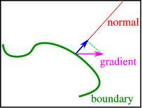
Typically we cannot specify the gradient at the boundary since that is too restrictive to allow for solutions. We can – and in physical problems often need to – specify the component normal to the boundary, see Figure \(\PageIndex{1}\) for an example. When this normal derivative is specified we speak of von Neumann boundary conditions.

In the case of an insulated (infinitely thin) rod of length \(a\), we can not have a heat-flux beyond the ends so that the gradient of the temperature must vanish (heat can only flow where a difference in temperature exists). This leads to the BC

\[\frac{\partial u}{\partial x}(0,t) = \frac{\partial u}{\partial x}(a,t) = 0. \nonumber \]

Mixed (Robin’s) Boundary Conditions

We can of course mix Dirichlet and von Neumann boundary conditions. For the thin rod example given above we could require

\[u(0,t) + \frac{\partial u}{\partial x}(0,t) = u(a,t) + \frac{\partial u}{\partial x}(a,t) = 0. \nonumber \]