
17.5: Degree Distribution
- Page ID
- 7875

Another local topological property that can be measured locally is, as we discussed already, the degree of a node. But if we collect them all for the whole network and represent them as a distribution, it will give us another important piece of information about how the network is structured:
A degree distribution of a network is a probability distribution
\[P(k) =\frac{| \begin{Bmatrix} i | deg(i) =k \end{Bmatrix}| }{ n}. \label{(17.28)} \]
i.e., the probability for a node to have degree \(k\).
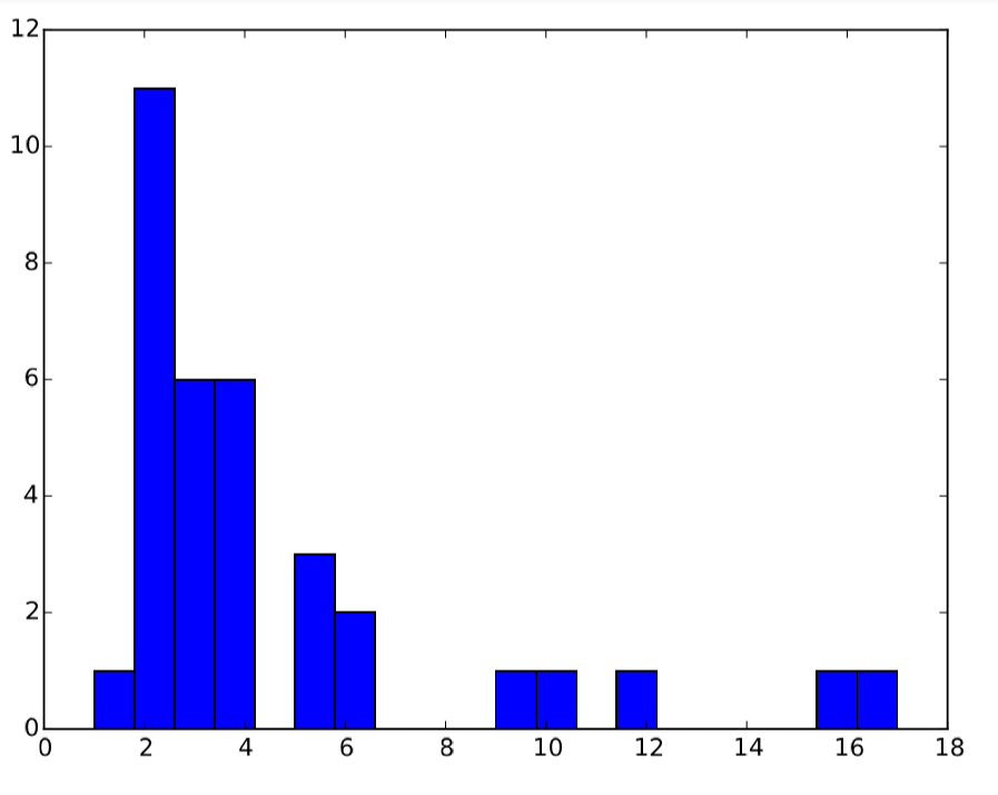
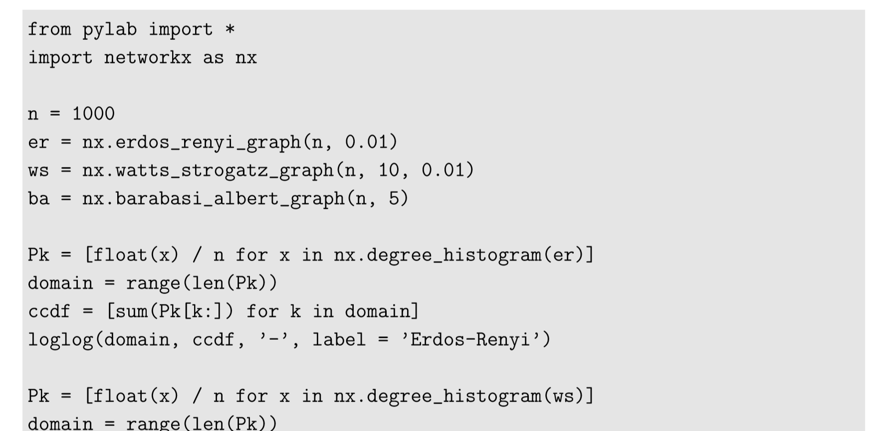
The degree distribution of a network can be obtained and visualized as follows:
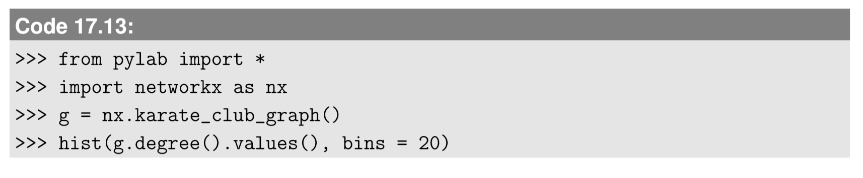
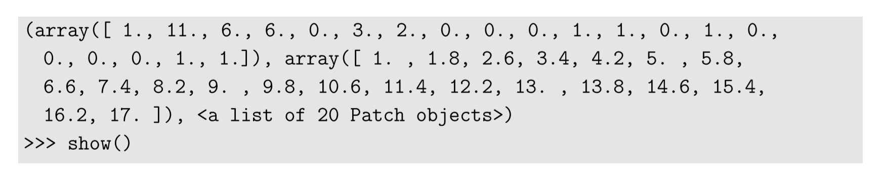
The result is shown in Fig. 17.5.1.
You can also obtain the actual degree distribution P(k) as follows:
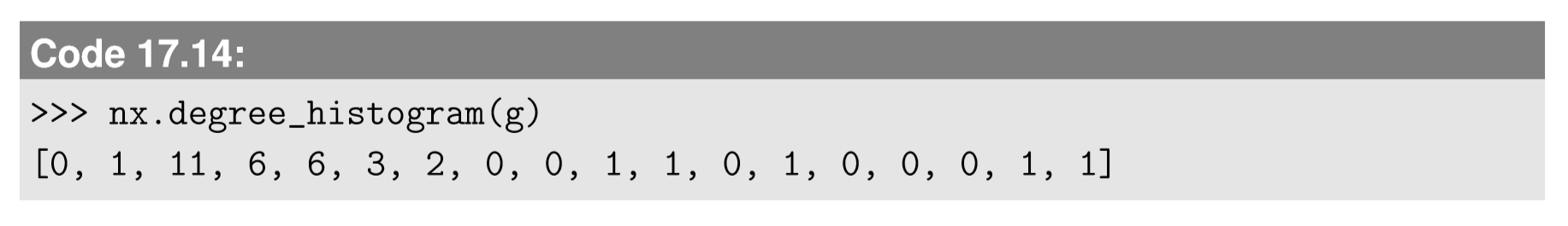
This list contains the value of (unnormalized) \(P(k) for k = 0,1,...,k_{max}\), in this order. For larger networks, it is often more useful to plot a normalized degree histogram list in a log-log scale:
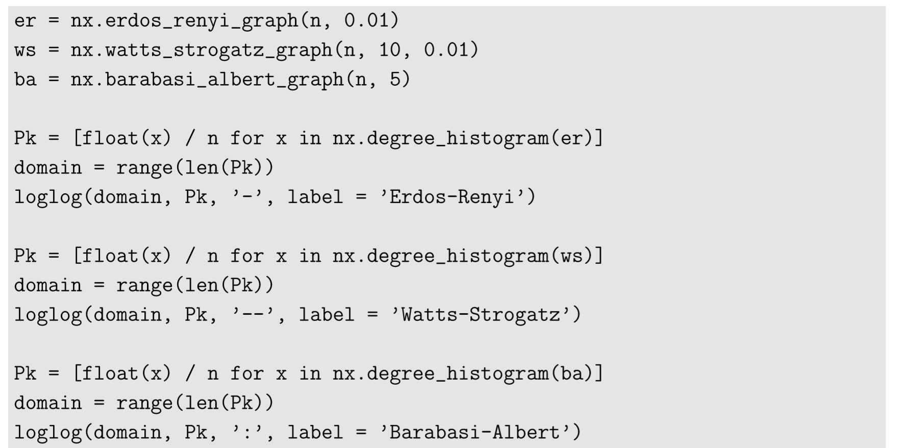
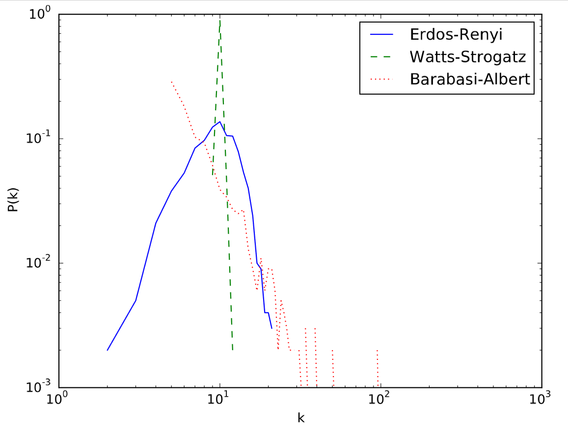
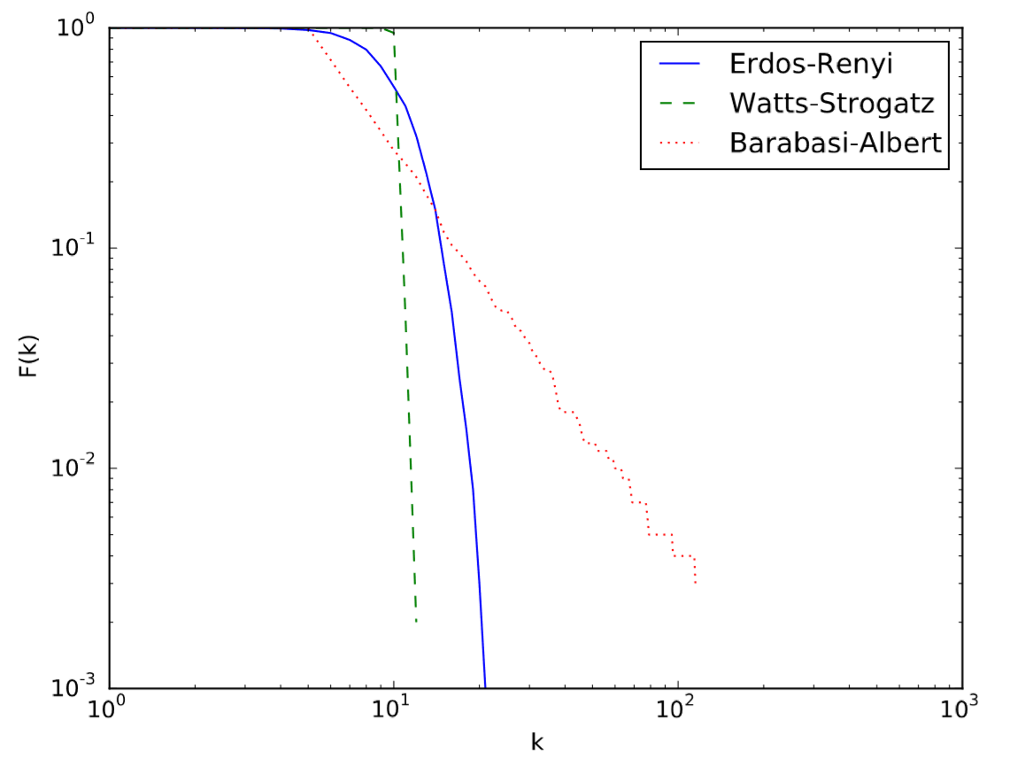
The result is shown in Fig. 17.5.2, which clearly illustrates differences between the three network models used in this example. The Erd˝os-R´enyi random network model has a bell-curved degree distribution, which appears as a skewed mountain in the log-log scale (blue solid line). The Watts-Strogatz model is nearly regular, and thus it has a very sharp peak at the average degree (green dashed line; \(k = 10\0 in this case). The Barab´asi-Albert model has a power-law degree distribution, which looks like a straight line with a negative slope in the log-log scale (red dotted line).
Moreover, it is often visually more meaningful to plot not the degree distribution itself but its complementary cumulative distribution function (CCDF), defined as follows:
\[F(k) =\sum_{k'=k} ^{\infty} P(k') \label{(17.29)} \]
This is a probability for a node to have a degree \(k\) or higher. By definition, \(F(0) = 1\) and \(F(k_{max} + 1) = 0\), and the function decreases monotonically along \(k\). We can revise Code 17.15 to draw CCDFs:


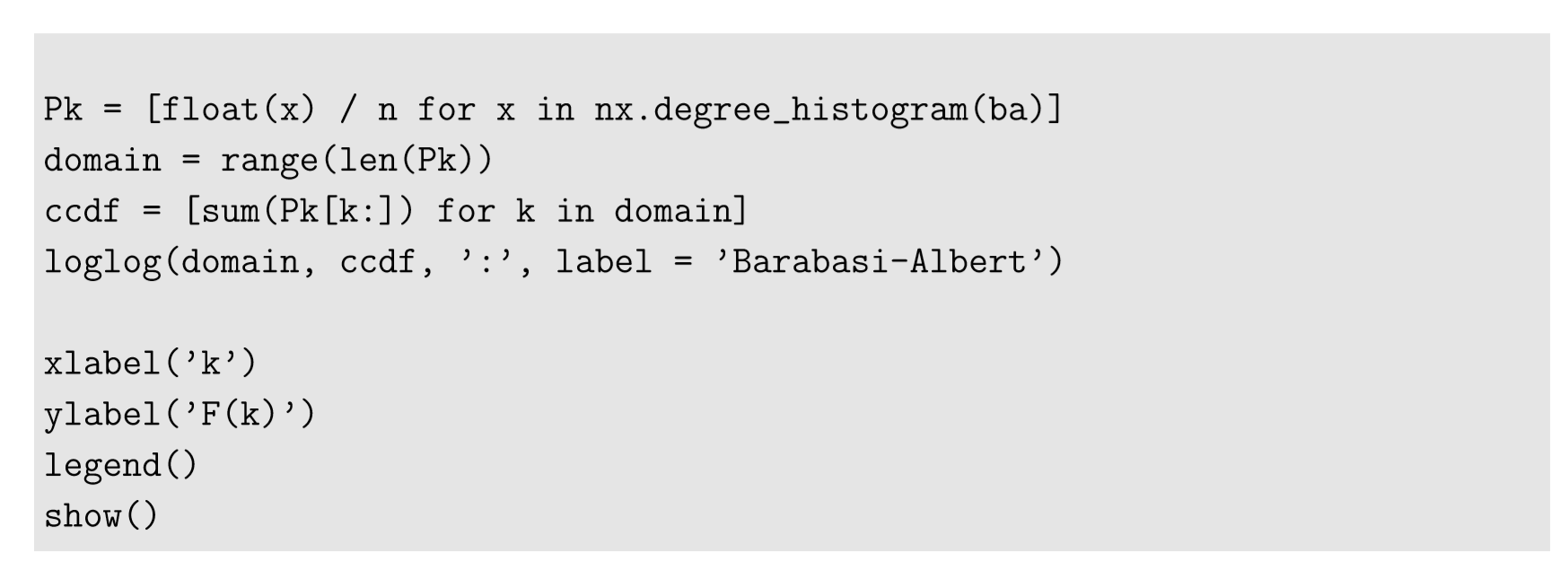
In this code, we generate ccdf’s from Pk by calculating the sum of Pk after dropping its first k entries. The result is shown in Fig. 17.5.2.
As you can see in the figure, the power law degree distribution remains as a straight line in the CCDF plot too, because \(F(k)\) will still be a power function of\( k\), as shown below:
\[F(k ) \begin{align} \sum_{k'=k} ^{\infty} {P(k')} = \sum_{k'=k} ^{infty}{ak' ^{-\gamma}} \label{(17.30)} \\ \approx \int_{k}^{infty} ak^{-\gamma}dk' = {\begin{bmatrix} \frac{ak^{J-\gamma+1}}{-\gamma + 1}\end{bmatrix}}^{\infty}_{k} = \frac{0-ak^{-\gamma+1}}{-\gamma +1} \label{(17.31)} \\ = \frac{a}{-\gamma -1}k ^{-(\gamma -1)} \label{(17.32)} \end{align} \]
This result shows that the scaling exponent of \(F(k)\) for a power law degree distribution is less than that of the original distribution by 1, which can be visually seen by comparing their slopes between Figs. 17.5.2 and 17.5.3.
Import a large network data set of your choice from Mark Newman’s Network Data website: http://www-personal.umich.edu/~mejn/netdata/
Plot the degree distribution of the network, as well as its CCDF. Determine whether the network is more similar to a random, a small-world, or a scale-free network model.
If the network’s degree distribution shows a power law behavior, you can estimate its scaling exponent from the distribution by simple linear regression. You should use a CCDF of the degree distribution for this purpose, because CCDFs are less noisy than the original degree distributions. Here is an example of scaling exponent estimation applied to a Barab´asi-Albert network, where the linregress function in SciPy’s stats module is used for linear regression:
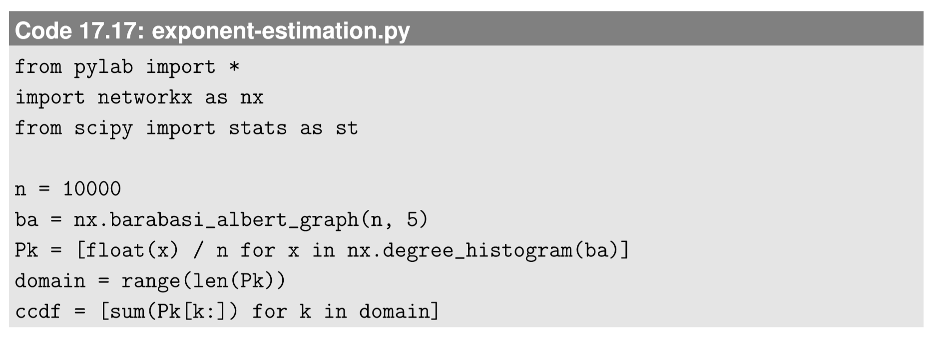
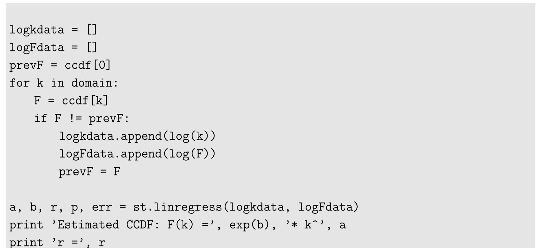
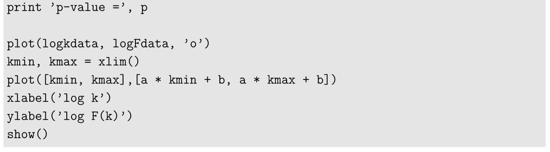
In the second code block, the domain and ccdf were converted to log scales for linear fitting. Also, note that the original ccdf contained values for all k’s, even for those for which \(P(k) = 0\). This would cause unnecessary biases in the linear regression toward the higher k end where actual samples were very sparse. To avoid this, only the data points where the value of \(F\) changed (i.e., where there were actual nodes with degree k) are collected in the logkdata and logFdata lists.
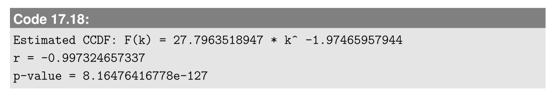
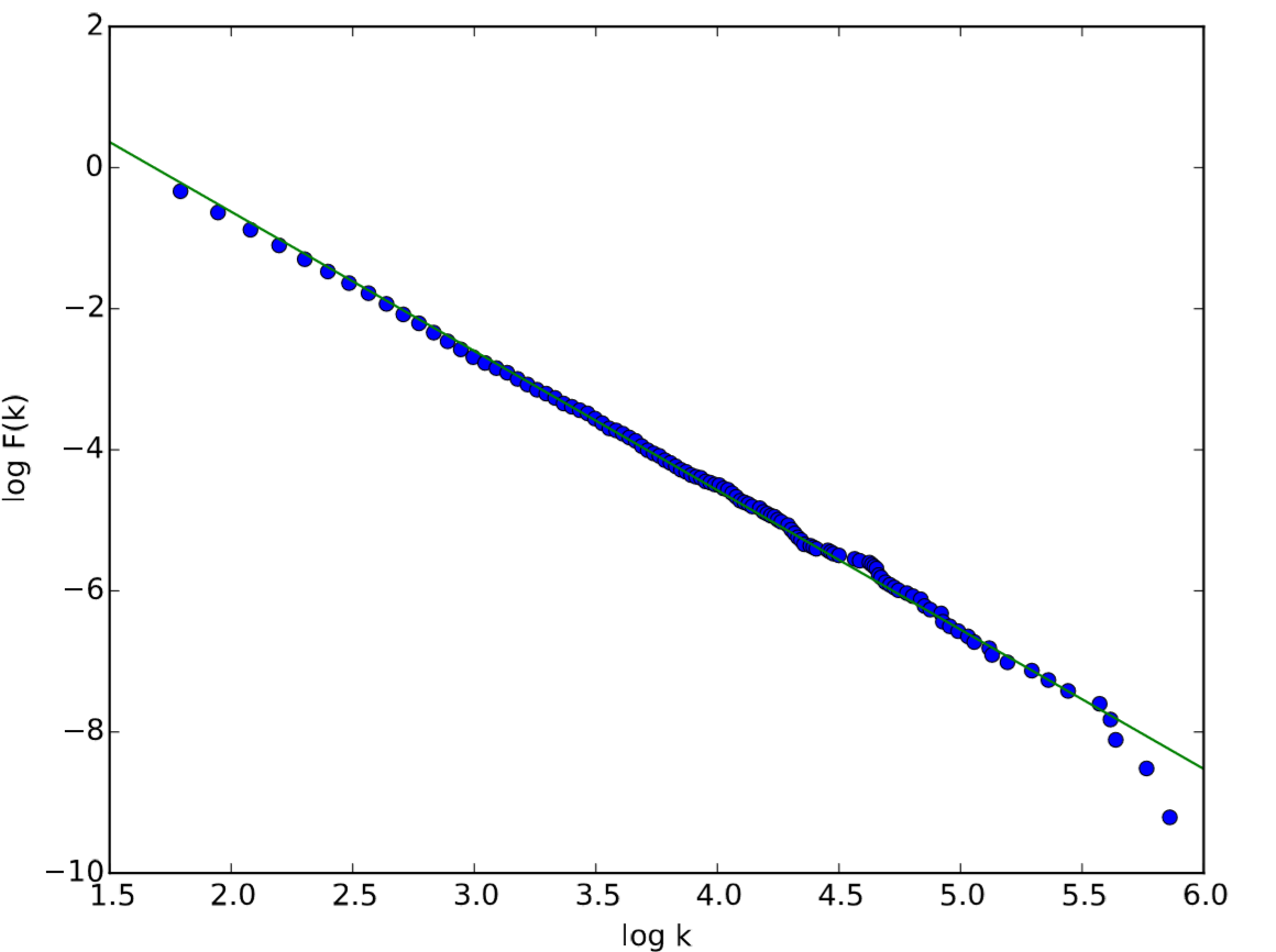
The result is shown in Fig. 17.5.4, and also the following output comes out to the terminal, which indicates that this was a pretty good fit:
Obtain a large network data set whose degree distribution appears to follow a power law, from any source (there are tons available online, including Mark Newman’s that was introduced before). Then estimate its scaling exponent using linear regression.