8.2: Polar Coordinates

Last updated
Save as PDF

Page ID: 13876

$ \newcommand{\vecs}[1]{\overset { \scriptstyle \rightharpoonup} {\mathbf{#1}} } $ $ \newcommand{\vecd}[1]{\overset{-\!-\!\rightharpoonup}{\vphantom{a}\smash {#1}}} $$\newcommand{\id}{\mathrm{id}}$ $ \newcommand{\Span}{\mathrm{span}}$ $ \newcommand{\kernel}{\mathrm{null}\,}$ $ \newcommand{\range}{\mathrm{range}\,}$ $ \newcommand{\RealPart}{\mathrm{Re}}$ $ \newcommand{\ImaginaryPart}{\mathrm{Im}}$ $ \newcommand{\Argument}{\mathrm{Arg}}$ $ \newcommand{\norm}[1]{\| #1 \|}$ $ \newcommand{\inner}[2]{\langle #1, #2 \rangle}$ $ \newcommand{\Span}{\mathrm{span}}$ $\newcommand{\id}{\mathrm{id}}$ $ \newcommand{\Span}{\mathrm{span}}$ $ \newcommand{\kernel}{\mathrm{null}\,}$ $ \newcommand{\range}{\mathrm{range}\,}$ $ \newcommand{\RealPart}{\mathrm{Re}}$ $ \newcommand{\ImaginaryPart}{\mathrm{Im}}$ $ \newcommand{\Argument}{\mathrm{Arg}}$ $ \newcommand{\norm}[1]{\| #1 \|}$ $ \newcommand{\inner}[2]{\langle #1, #2 \rangle}$ $ \newcommand{\Span}{\mathrm{span}}$$\newcommand{\AA}{\unicode[.8,0]{x212B}}$

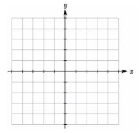
The coordinate system we are most familiar with is called the Cartesian coordinate system, a rectangular plane divided into four quadrants by horizontal and vertical axes.

$An empty rectangular coordinate grid, with horizontal and vertical grid lines.$ In earlier chapters, we often found the Cartesian coordinates of a point on a circle at a given angle from the positive horizontal axis. Sometimes that angle, along with the point’s distance from the origin, provides a more useful way of describing the point’s location than conventional Cartesian coordinates.

POLAR COORDINATES

Polar coordinates of a point consist of an ordered pair, ($r$,$\theta$), where $r$ is the distance from the point to the origin, and $\theta$ is the angle measured in standard position.

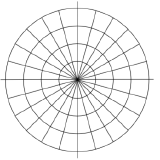
$An empty polar graphing grid, with concentric circles centered at the origin, and rays drawn from the origin at incremental angles.$

Notice that if we were to “grid” the plane for polar coordinates, it would look like the graph to the right, with circles at incremental radii, and rays drawn at incremental angles.

Example $\PageIndex{1}$

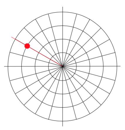
Plot the polar point ($3, \dfrac{5\pi}{6}$).

Solution

This point will be a distance of 3 from the origin, at an angle of $\dfrac{5\pi}{6}$. Plotting this

$A polar grid, with a point A in the first quadrant$

Example $\PageIndex{2}$

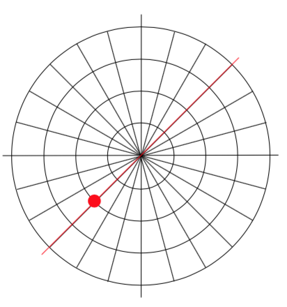
Plot the polar point ($-2, \dfrac{\pi}{4}$).

Solution

Typically we use positive $r$ values, but occasionally we run into cases where $r$ is negative. On a regular number line, we measure positive values to the right and negative values to the left. We will plot this point similarly. To start, we rotate to an angle of $\dfrac{\pi}{4}$.

Moving this direction, into the first quadrant, would be positive rvalues. For negative r values, we move the opposite direction, into the third quadrant. Plotting this:

$On a polar grid, a line is shown at an angle of pi over 4, with a point indicated on the line in the third quadrant a distance of 2 from the origin.$

Note the resulting point is the same as the polar point ($2, \dfrac{5\pi}{4}$). In fact, any Cartesian point can be represented by an infinite number of different polar coordinates by adding or subtracting full rotations to these points. For example, same point could also be represented as ($2, \dfrac{13\pi}{4}$).

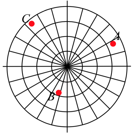
Exercise $\PageIndex{1}$

Plot the following points given in polar coordinates and label them.

a. $A = (3, \dfrac{\pi}{6})$

b. $B = (-2, \dfrac{\pi}{3})$

c. $C = (4, \dfrac{3\pi}{4})$

Answer: $A polar grid. Point A is on the radius 3 circle at angle pi over 6 in the first quadrant. Point B is on the radius 2 circle in the third quadrant at angle 4 pi over 3. Point C is on the radius 4 circle in the second quadrant at angle 3 pi over 4.$

Converting Points

To convert between polar coordinates and Cartesian coordinates, we recall the relationships we developed back in Chapter 5.

CONVERTING BETWEEN POLAR AND CARTESIAN COORDINATES

To convert between polar ($r, \theta$) and Cartesian ($x, y$) coordidates, we use the relationships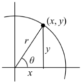 $A circle centered at the origin with a line labeled r drawn at an angle of theta. The point where the line meets the circle is labeled x comma y. A vertical line is drawn from that point to the x axis forming a triangle, with the vertical length labeled y. The horizontal leg of the triangle from the origin to the vertical line is labeled x.$

\[\cos (\theta )=\frac{x}{r}\quad x=r\cos (\theta )\]

\[\sin (\theta )=\frac{y}{r}\quad y=r\sin (\theta )\]

\[\tan (\theta )=\frac{y}{x}\quad x^{2}+y^{2}=r^{2}\]

From these relationship and our knowledge of the unit circle, if $r = 1$ and $\theta = \dfrac{\pi}{3}$, the polar coordinates would be $(r, \theta) = (1, \dfrac{\pi}{3})$, and the corresponding Cartesian coordinates $(x, y) = (\dfrac{1}{2}, \dfrac{\sqrt{3}}{2})$.

Remembering your unit circle values will come in very handy as you convert between Cartesian and polar coordinates.

Example $\PageIndex{3}$

Find the Cartesian coordinates of a point with polar coordinates $(r, \theta) = (5, \dfrac{2\pi}{3})$.

Solution

To find the $x$ and $y$ coordinates of the point,

\[x = r\text{cos} (\theta) = 5 \cos (\dfrac{2\pi}{3}) = 5(-\dfrac{1}{2}) = -\dfrac{5}{2}\nonumber\]

\[y = r\text{sin} (\theta) = 5 \sin (\dfrac{2\pi}{3}) = 5(-\dfrac{\sqrt{3}}{2}) = -\dfrac{5\sqrt{3}}{2}\nonumber\]

The Cartesian coordinates are ($-\dfrac{5}{2}, \dfrac{5\sqrt{3}}{2}$).

Example $\PageIndex{4}$

Find the polar coordinates of the point with Cartesian coordinates (−3,−4) .

Solution

We begin by finding the distance $r$ using the Pythagorean relationship $x^2 + y^2 = r^2$

\[(-3)^2 + (-4)^2 = r^2\nonumber\]
\[9 + 16 = r^2\nonumber\]
\[r^2 = 25\nonumber\]
\[r = 5\nonumber\]

Now that we know the radius, we can find the angle using any of the three trig relationships. Keep in mind that any of the relationships will produce two solutions on the circle, and we need to consider the quadrant to determine which solution to accept. Using the cosine, for example:

\[\cos(\theta) = \dfrac{x}{r} = \dfrac{-3}{5}\nonumber\]
\[\theta = \cos^{-1}(\dfrac{-3}{5}) \approx 2.214\nonumber\]By symmetry, there is a second possibility at
\[\theta = 2\pi - 2.24 = 4.069\nonumber\]

Since the point (-3, -4) is located in the $3^{\text{rd}}$ quadrant, we can determine that the second angle is the one we need. The polar coordinates of this point are $(r, \theta) = (5, 4.069)$.

Exercise $\PageIndex{2}$

Convert the following.

a. Convert polar coordinates $(r, \theta) = (2, \pi)$ to ($x, y)$.

b. Convert Cartesian coordinates $(x, y) = (0, -4)$ to $(r, \theta)$.

Answer

a. $(r, \theta) = (2, \pi)$ converts to $(x, y) = (2\cos(\pi), 2\sin(\pi)) = (-2, 0)$

b. $(x, y) = (0, -4)$ converts to $(r, \theta) = (4, \dfrac{3\pi}{2})\ or\ (-4, \dfrac{\pi}{2})$

Polar Equations

Just as a Cartesian equation like $y = x^2$ describes a relationship between $x$ and $y$ values on a Cartesian grid, a polar equation can be written describing a relationship between $r$ and $\theta$ values on the polar grid.

Example $\PageIndex{5}$

Sketch a graph of the polar equation $r = \theta$.

Solution

The equation $r = \theta$ describes all the points for which the radius $r$ is equal to the angle. To visualize this relationship, we can create a table of values.

$\theta$	0	$\pi/4$	$\pi/2$	$3\pi/4$	$\pi$	$5\pi/4$	$3\pi/2$	$7\pi/4$	$2\pi$
$r$	0	$\pi/4$	$\pi/2$	$3\pi/4$	$\pi$	$5\pi/4$	$3\pi/2$	$7\pi/4$	$2\pi$

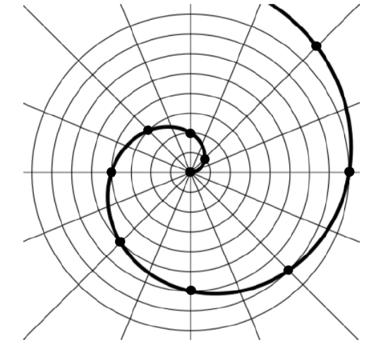
$On a polar grid, a graph that spirals out from the origin. At an angle of pi over 4 there is a point a distance pi over 4 from the origin. At an angle of pi over 2 there's a point a distance pi over 2 from the origin, and so on.$

We can plot these points on the plane, and then sketch a curve that fits the points. The resulting graph is a spiral.

Notice that the resulting graph cannot be the result of a function of the form $y = f(x)$, as it does not pass the vertical line test, even though it resulted from a function giving $r$ in terms of $\theta$.

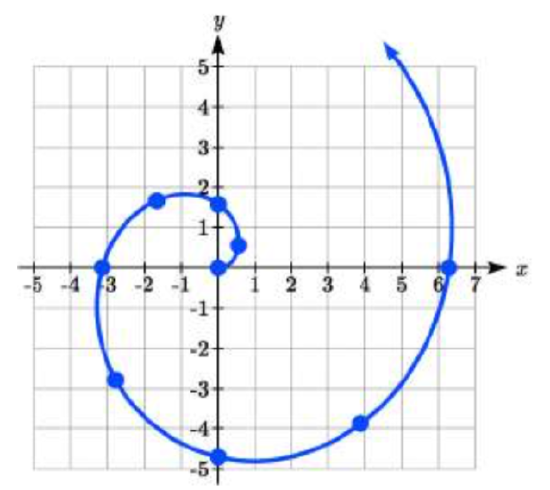
$A spiral graph shown on a cartesian grid. The graph spirals out from the origin, passing through these approximate points: 0 comma 0, 0.5 comma 0.5, 0 comma 1.6, negative 1.6 comma 1.6, negative pi comma 0, negative 2.9 comma neative 2.9, 0 comma negative 4.8.$

Although it is nice to see polar equations on polar grids, it is more common for polar graphs to be graphed on the Cartesian coordinate system, and so, the remainder of the polar equations will be graphed accordingly.

The spiral graph above on a Cartesian grid is shown here.

Example $\PageIndex{6}$

Sketch a graph of the polar equation $r = 3$.

Solution

Recall that when a variable does not show up in the equation, it is saying that it does not matter what value that variable 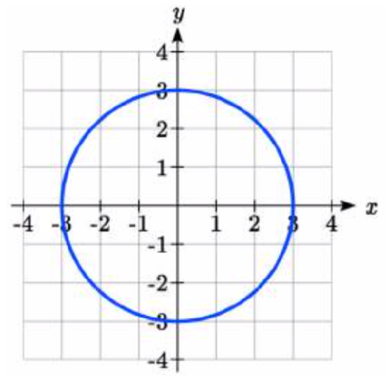$A circle with radius 3 centered at the origin.$ has; the output for the equation will remain the same. For example, the Cartesian equation $y = 3$ describes all the points where $y = 3$, no matter what the x values are, producing a horizontal line.

Likewise, this polar equation is describing all the points at a distance of 3 from the origin, no matter what the angle is, producing the graph of a circle.

The normal settings on graphing calculators and software graph on the Cartesian coordinate system with $y$ being a function of $x$, where the graphing utility asks for $f(x)$, or simply $y =$.

To graph polar equations, you may need to change the mode of your calculator to Polar. You will know you have been successful in changing the mode if you now have $r$ as a function of $\theta$, where the graphing utility asks for $r(\theta)$, or simply $r =$.

Example $\PageIndex{7}$

Sketch a graph of the polar equation $r = 4 \cos(\theta)$, and find an interval on which it completes one cycle.

Solution

While we could again create a table, plot the corresponding points, and connect the dots, we can also turn to technology to directly graph it. Using technology, we produce the graph shown here, a circle passing through the origin.

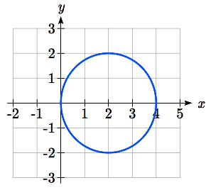
$A circle with radius 2, centered at 2 comma 0. The graph touches the points 0 comma 0 and 4 comma 0.$

Since this graph appears to close a loop and repeat itself, we might ask what interval of $\theta$ values yields the entire graph. At $\theta = 0$, $r = 4\cos(0) = 4$, yielding the point (4, 0). We want the next $\theta$ value when the graph returns to the point (4, 0). Solving for when $x = 4$ is equivalent to solving $r\cos(\theta) = 4$.

\[r \cos(\theta) = 4\nonumber\]Substituting the equation for $r$ gives
\[4\cos(\theta)\cos(\theta) = 4\nonumber\]Dividing by 4 and simplifying
\[\cos^{2}(\theta)= 1\nonumber\]This has solutions when
\[\cos(\theta) = 1\text{ or }\cos(\theta) = -1\nonumber\]Solving these gives solutions
\[\theta = 0\text{ or }\theta = \pi\nonumber\]

This shows us at 0 radians we are at the point (0, 4), and again at $\pi$ radians we are at the point (0, 4) having finished one complete revolution.

This interval $0 \le \theta < \pi$ yields one complete iteration of the circle.

Exercise $\PageIndex{3}$

Sketch a graph of the polar equation $r = 3 \sin (\theta)$, and find an interval on which it completes one cycle.

Answer

\[3 \sin(\theta) = 0\text{ at }\theta = 0\text{ and }\theta = \pi\nonumber\]

It completes one cycle on the interval $0 \le \theta < \pi$.

$A circle with radius 1.5, centered at 0 comma 1.5. The circle touches the origin and the point 0 comma 3.$

The last few examples have all been circles. Next, we will consider two other “named” polar equations, limaçons and roses.

Example $\PageIndex{8}$

Sketch a graph of the polar equation $r = 4\sin(\theta) + 2$. What interval of $\theta$ values corresponds to the inner loop?

Solution

This type of graph is called a limaçon.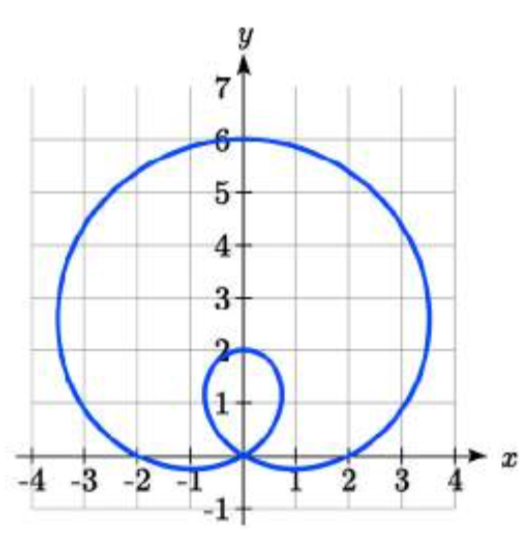 $A graph of a limacon. The graph has a large rounded loop, starting at the origin, dipping down then increasing through 2 comma 0, looping up to 0 comma 6, looping to negative 2 comma 0 then circling back to the origin. The graph then continues in a small loop which also starts at the origin, loops up to 0 comma 2, then back to the origin.$
Using technology, we can draw the graph. The inner loop begins and ends at the origin, where $r = 0$. We can solve forthe $\theta$ values for which $r = 0$.

\[0 = 4\sin(\theta) + 2\nonumber\]
\[-2 = 4\sin(\theta)\nonumber\]
\[\sin(\theta) = -\dfrac{1}{2}\nonumber\]
\[\theta = \dfrac{7\pi}{6}\text{ or }\theta = \dfrac{11\pi}{6}\nonumber\]

This tells us that $r = 0$, so the graph passes through the origin, twice on the interval $[0, 2\pi)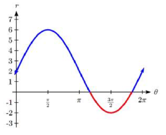$. $The horizontal axis is labeled theta and the vertical axis labeled r. A sinusoidal graph, starting at the midline at 0 comma 2, increasing up to pi over 2 comma 6, decreasing down to 3 pi over 2 comma negative 2, then increasing back up to 2 pi comma 2. The portion of the graph that has a negative output is highlighted in red$

The inner loop arises from the interval $\dfrac{7\pi}{6} \le \theta \le \dfrac{11\pi}{6}$.

This corresponds to where the function $r = 4 \sin(\theta) + 2$ takes on negative values, as we could see if we graphed the function in the $r \theta$ plane.

Example $\PageIndex{9}$

Sketch a graph of the polar equation $r = \cos(3\theta)$. What interval of $\theta$ values describes one small loop of the graph?

Solution

This type of graph is called a 3 leaf rose. 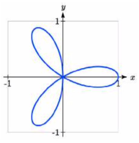$A graph of a 3 leaf rose. The graph consists of 3 loops, all touching the origin. The first loop is furthest from the origin at 1 comma 0. The second is furthest at negative one half comma square root of 3 over 2. The third is furthest at negative one half comma negative square root of 3 over 2.$

We can use technology to produce a graph. The interval $[0, \pi)$ yields one cycle of this function. As with the last problem, we can note that there is an interval on which one loop of this graph begins and ends at the origin, where $r = 0$. Solving for $\theta$,

\[0 = \cos(3\theta)\nonumber\]Substitute $u = 3\theta$
\[0 = \cos(u)\nonumber\]
\[u = \dfrac{\pi}{2}\text{ or }u = \dfrac{3\pi}{2}\text{ or }u = \dfrac{5\pi}{2}\nonumber\]

Undo the substitution,

\[3 \theta = \dfrac{\pi}{2}\text{ or }3 \theta = \dfrac{3\pi}{2}\text{ or }3 \theta = \dfrac{5\pi}{2}\nonumber\]

\[\theta = \dfrac{\pi}{6}\text{ or }\theta = \dfrac{\pi}{2}\text{ or }\theta = \dfrac{5\pi}{6}\nonumber\]

There are 3 solutions on $0 \le \theta < \pi$ which correspond to the 3 times the graph returns to the origin, but the first two solutions we solved for above are enough to conclude that

one loop corresponds to the interval $\dfrac{\pi}{6} \le \theta < \dfrac{\pi}{2}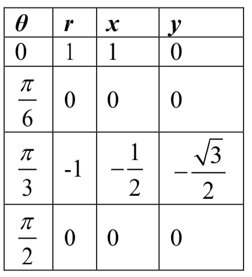$. $屏幕快照 2019-07-21 上午7.54.40.png$

If we wanted to get an idea of how the computer drew this graph, consider when $\theta = 0$.

$r = \cos(3\theta) = \cos(0) = 1$, so the graph starts at (1, 0). As we found above, at $\theta = \dfrac{\pi}{6}$ and $\theta = \dfrac{\pi}{2}$, the graph is at the origin. Looking at the equation, notice that any angle in between $\dfrac{\pi}{6}$ and $\dfrac{\pi}{2}$, for example at $\theta = \dfrac{\pi}{3}$, produces a negative $r$: \[r = \cos(3 \cdot \dfrac{\pi}{3}) = \cos(\pi) = -1\nonumber\]

Notice that with a negative $r$ value and an angle with terminal side in the first quadrant, the corresponding Cartesian point would be in the third quadrant. Since $r = \cos(3\theta)$ is negative on $\dfrac{\pi}{6} \le \theta < \dfrac{\pi}{2}$, this interval corresponds to the loop of the graph in the third quadrant.

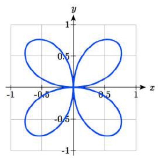
Exercise $\PageIndex{4}$

Sketch a graph of the polar equation $r = \sin(2\theta)$. Would you call this function alimaçon or a rose?

Answer

This is a 4-leaf rose.

$A graph of a 4 leaf rose, consisting of 4 loops, all touching the origin. The first loop is furthest from the origin at square root of 2 comma square root of 2, and the other 3 leafs are reflections of that one across the axes and the origin.$

Converting Equations

While many polar equations cannot be expressed nicely in Cartesian form (and vice versa), it can be beneficial to convert between the two forms, when possible. To do this we use the same relationships we used to convert points between coordinate systems.

Example $\PageIndex{10}$

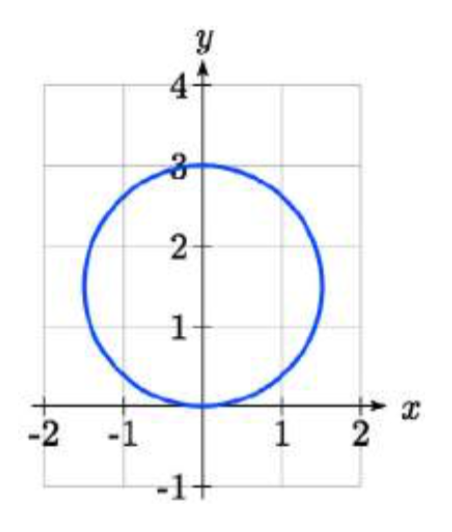
Rewrite the Cartesian equation $x^2 + y^2 = 6y$ as a polar equation.

Solution

We wish to eliminate $x$ and $y$ from the equation and introduce $r$ and $\theta$. Ideally, we would like to write the equation with $r$ isolated, if possible, which represents $r$ as a function of $\theta$.

\[x^2 + y^2 = 6y\nonumber\]Remembering $x^2 + y^2 = r^2$ we substitute
\[r^2 = 6y\nonumber\] $y = r\sin(\theta)$ and so we substitute again
\[r^2 = 6r \sin(\theta)\nonumber\] Subtract $6r\sin(\theta)$ from both sides
\[r^2 - 6r\sin(\theta) = 0\nonumber\]Factor
\[r (r - 6\sin(\theta)) = 0\nonumber\] Use the zero factor theorem
\[r = 6\sin(\theta)\text{ or }r = 0\nonumber\] Since $r = 0$ is only a point, we reject that solution.

The solution $r = 6\sin(\theta)$ is fairly similar to the one we graphed in Example 7. In fact, this equation describes a circle with bottom at the origin and top at the point (0, 6).

Example $\PageIndex{11}$

Rewrite the Cartesian equation $y = 3x + 2$ as a polar equation.

Solution

\[y = 3x + 2\nonumber\]Use $y = r\sin(\theta)$ and $x = r\cos(\theta)$
\[r\sin(\theta) = 3r\cos(\theta) + 2\nonumber\] Move all terms with $r$ to one side
\[r\sin(\theta) - 3r\cos(\theta) = 2\nonumber\] Factor out $r$
\[r(\sin(\theta) - 3\cos(\theta)) = 2\nonumber\] Divide
\[r = \dfrac{2}{\sin(\theta) - 3\cos(\theta)}\nonumber\]

In this case, the polar equation is more unwieldy than the Cartesian equation, but there are still times when this equation might be useful.

Example $\PageIndex{12}$

Rewrite the polar equation $r = \dfrac{3}{1- 2\cos(\theta)}$ as a Cartesian equation.

Solution

We want to eliminate $\theta$ and $r$ and introduce $x$ and $y$. It is usually easiest to start by clearing the fraction and looking to substitute values that will eliminate $\theta$.

\[r = \dfrac{3}{1 - 2\cos(\theta)}\nonumber\]Clear the fraction
\[r(1 - 2\cos(\theta)) = 3\nonumber\]Use $\cos(\theta) = \dfrac{x}{r}$ to eliminate $\theta$
\[r(1 - 2\dfrac{x}{r}) = 3\nonumber\] Distribute and simplify
\[r - 2x = 3\nonumber\] Isolate the $r$
\[r = 3 + 2x\nonumber\] Square both sides
\[r^2 = (3 + 2x)^2\nonumber\] Use $x^2 + y^2 = r^2$
\[x^2 + y^2 = (3+2x)^2\nonumber\]

When our entire equation has been charged from $r$ and $\theta$ to $x$ and $y$ we can stop unless asked to solve for $y$ or simplify.

In this example, if desired, the right side of the equation could be expanded and the equation simplified further. However, the equation cannot be written as a function in Cartesian form.

Exercise $\PageIndex{5}$

a. Rewrite the Cartesian equation in polar form: $y = \pm \sqrt{3 - x^2}$

b. Rewrite the polar equation in Cartesian form: $r = 2\sin(\theta)$

Answer

a. $y = \pm \sqrt{3 - x^2}$ can be rewritten as $x^2 + y^2 = 3$, and becomes $r = \sqrt{3}$

b. \[r = 2\sin(\theta)\nonumber\]
\[r= 2\dfrac{y}{r}\nonumber\]
\[r^2 = 2y\nonumber\]
\[x^2 + y^2 = 2y\nonumber\]

Example $\PageIndex{13}$

Rewrite the polar equation $r = \sin(2\theta)$ in Cartesian form.

Solution

\[r = \sin(2\theta)\nonumber\] Use the double angle identity for sine
\[r = 2\sin(\theta)\cos(\theta)\nonumber\] Use $\cos(\theta) = \dfrac{x}{r}$ and $\sin(\theta) = \dfrac{y}{r}$
\[r = 2 \cdot \dfrac{x}{r} \cdot \dfrac{y}{r}\nonumber\] Simplify
\[r = \dfrac{2xy}{r^2}\nonumber\]Multiply by $r^2$
\[r^3 = 2xy\nonumber\]Since $x^2 + y^2 = r^2$, $r = \sqrt{x^2 + y^2}$
\[(\sqrt{x^2 + y^2})^3 = 2xy\nonumber\]

This equation could also be written as

\[(x^2 + y^2)^{3/2} = 2xy\text{ or }x^2 + y^2 = (2xy)^{2/3}\nonumber\]

Important Topics of This Section

Cartesian coordinate system
Polar coordinate system
Plotting points in polar coordinates
Converting coordinates between systems
Polar equations: Spirals, circles, limaçons and roses Converting equations between systems

\(\theta\)	0	\(\pi/4\)	\(\pi/2\)	\(3\pi/4\)	\(\pi\)	\(5\pi/4\)	\(3\pi/2\)	\(7\pi/4\)	\(2\pi\)
\(r\)	0	\(\pi/4\)	\(\pi/2\)	\(3\pi/4\)	\(\pi\)	\(5\pi/4\)	\(3\pi/2\)	\(7\pi/4\)	\(2\pi\)