
1.5: Some Algorithms of Elementary Number Theory
- Page ID
- 19364

An algorithm is simply a set of clear instructions for achieving some task. The Persian mathematician and astronomer Al-Khwarizmi1 was a scholar at the House of Wisdom in Baghdad who lived in the \(8^{\text{th}}\) and \(9^{\text{th}}\) centuries A.D. He is remembered for his algebra treatise Hisab al-jabr w’al-muqabala from which we derive the very word “algebra,” and a text on the Hindu-Arabic numeration scheme.
Al-Khwarizmi also wrote a treatise on Hindu-Arabic numerals. The Arabic text is lost but a Latin translation, Algoritmi de numero Indorum (in English Al-Khwarizmi on the Hindu Art of Reckoning) gave rise to the word algorithm deriving from his name in the title. [12]
While the study of algorithms is more properly a subject within Computer Science, a student of Mathematics can derive considerable benefit from it.
There is a big difference between an algorithm description intended for human consumption and one meant for a computer2. The two favored humanreadable forms for describing algorithms are pseudocode and flowcharts. The former is text-based and the latter is visual. There are many different modules from which one can build algorithmic structures: for-next loops, do-while loops, if-then statements, goto statements, switch-case structures, etc. We’ll use a minimal subset of the choices available.
- Assignment statements
- If-then control statements
- Goto statements
- Return
We take the view that an algorithm is something like a function, it takes for its input a list of parameters that describe a particular case of some general problem, and produces as its output a solution to that problem. (It should be noted that there are other possibilities – some programs require that the variable in which the output is to be placed be handed them as an input parameter, others have no specific output, their purpose is achieved as a side-effect.) The intermediary between input and output is the algorithm instructions themselves and a set of so-called local variables which are used much the way scrap paper is used in a hand calculation – intermediate calculations are written on them, but they are tossed aside once the final answer has been calculated.
Assignment statements allow us to do all kinds of arithmetic operations (or rather to think of these types of operations as being atomic.) In actuality even a simple procedure like adding two numbers requires an algorithm of sorts, we’ll avoid such a fine level of detail. Assignments consist of evaluating some (possibly quite complicated) formula in the inputs and local variables and assigning that value to some local variable. The two uses of the phrase “local variable” in the previous sentence do not need to be distinct, thus \(x = x + 1\) is a perfectly legal assignment.
If-then control statements are decision makers. They first calculate a Boolean expression (this is just a fancy way of saying something that is either true or false), and send program flow to different locations depending on that result. A small example will serve as an illustration. Suppose that in the body of an algorithm we wish to check if \(2\) variables, \(x\) and \(y\) are equal, and if they are, increment \(x\) by \(1\). This is illustrated in Figure \(1.5.1\) both in pseudocode and as a flowchart.
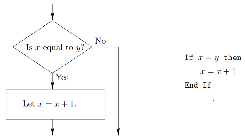
Notice the use of indentation in the pseudocode example to indicate the statements that are executed if the Boolean expression is true. These examples also highlight the difference between the two senses that the word “equals” (and the symbol \(=\)) has. In the Boolean expression, the sense is that of testing equality, in the assignment statements (as the name implies) an assignment is being made. In many programming languages, this distinction is made explicit, for instance in the C language equality testing is done via the symbol “\(==\)” whereas assignment is done using a single equals sign (\(=\)). In Mathematics the equals sign usually indicates equality testing, when the assignment sense is desired the word “let” will generally precede the equality.
While this brief introduction to the means of notating algorithms is by no means complete, it is hopefully sufficient for our purpose which is solely to introduce two algorithms that are important in elementary number theory. The division algorithm, as presented here, is simply an explicit version of the process one follows to calculate a quotient and remainder using long division. The procedure we give is unusually inefficient – with very little thought one could devise an algorithm that would produce the desired answer using many fewer operations – however the main point here is purely to show that division can be accomplished by essentially mechanical means. The Euclidean algorithm is far more interesting both from a theoretical and a practical perspective. The Euclidean algorithm computes the greatest common divisor (\(\text{gcd}\)) of two integers. The \(\text{gcd}\) of of two numbers \(a\) and \(b\) is denoted \(\text{gcd}(a, b)\) and is the largest integer that divides both \(a\) and \(b\) evenly.
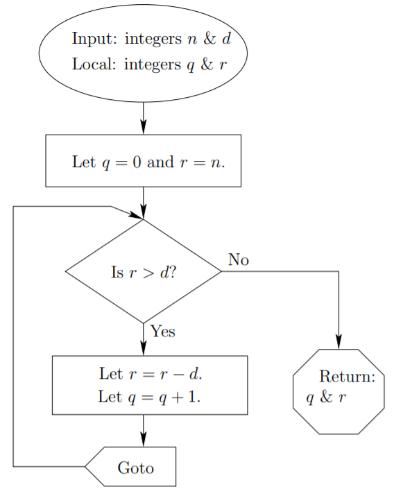
A pseudocode outline of the division algorithm is as follows:
Algorithm: Division
Inputs: integers \(n\) and \(d\).
Local variables: \(q\) and \(r\).
Let \(q = 0\).
Let \(r = n\).
Label \(1\).
If \(r < d\) then
Return \(q\) and \(r\).
End If
Let \(q = q + 1\).
Let \(r = r − d\).
Goto \(1\).
This same algorithm is given in flowchart form in Figure \(1.5.2\).
Note that in a flowchart the action of a “Goto” statement is clear because an arrow points to the location where program flow is being redirected. In pseudocode a “Label” statement is required which indicates a spot where flow can be redirected via subsequent “Goto” statements. Because of the potential for confusion in complicated algorithms that involve multitudes of Goto statements and their corresponding Labels, this sort of redirection is now deprecated in virtually all popular programming environments.
Before we move on to describe the Euclidean algorithm it might be useful to describe more explicitly what exactly it’s for. Given a pair of integers, \(a\) and \(b\), there are two quantities that it is important to be able to compute, the least common multiple or \(\text{lcm}\), and the greatest common divisor or \(\text{gcd}\). The \(\text{lcm}\) also goes by the name lowest common denominator because it is the smallest denominator that could be used as a common denominator in the process of adding two fractions that had \(a\) and \(b\) in their denominators. The \(\text{gcd}\) and the \(\text{lcm}\) are related by the formula
\[\text{lcm}(a,b) = \dfrac{ab}{\text{gcd}(a, b)} \]
so they are essentially equivalent as far as representing a computational challenge.
The Euclidean algorithm depends on a rather extraordinary property of the \(\text{gcd}\). Suppose that we are trying to compute \(\text{gcd}(a, b)\) and that \(a\) is the larger of the two numbers. We first feed \(a\) and \(b\) into the division algorithm to find \(q\) and \(r\) such that \(a = qb + r\). It turns out that \(b\) and \(r\) have the same gcd as did \(a\) and \(b\). In other words, \(\text{gcd}(a, b) = \text{gcd}(b, r)\), furthermore these numbers are smaller than the ones we started with! This is nice because it means we’re now dealing with an easier version of the same problem. In designing an algorithm it is important to formulate a clear ending criterion, a condition that tells you you’re done. In the case of the Euclidean algorithm, we know we’re done when the remainder \(r\) comes out \(0\).
So, here, without further ado is the Euclidean algorithm in pseudocode.
Algorithm: Euclidean
Inputs: integers \(a\) and \(b\).
Local variables: \(q\) and \(r\).
Label \(1\).
Let \((q, r)\) = Division\((a, b)\).
If \(r = 0\) then
Return \(b\).
End If
Let \(a = b\).
Let \(b = r\).
Goto \(1\).
It should be noted that for small numbers one can find the \(\text{gcd}\) and \(\text{lcm}\) quite easily by considering their factorizations into primes. For the moment consider numbers that factor into primes but not into prime powers (that is, their factorizations don’t involve exponents). The \(\text{gcd}\) is the product of the primes that are in common between these factorizations (if there are no primes in common it is \(1\)). The \(\text{lcm}\) is the product of all the distinct primes that appear in the factorizations. As an example, consider \(30\) and \(42\). The factorizations are \(30 = 2 · 3 · 5\) and \(42 = 2 · 3 · 7\). The primes that are common to both factorizations are \(2\) and \(3\), thus \(\text{gcd}(30, 42) = 2 · 3 = 6\). The set of all the primes that appear in either factorization is \(\{2, 3, 5, 7\}\) so \(\text{lcm}(30, 42) = 2 · 3 · 5 · 7 = 210\).
The technique just described is of little value for numbers having more than about \(50\) decimal digits because it rests a priori on the ability to find the prime factorizations of the numbers involved. Factoring numbers is easy enough if they’re reasonably small, especially if some of their prime factors are small, but in general the problem is considered so difficult that many cryptographic schemes are based on it.
Exercises
Trace through the division algorithm with inputs \(n = 27\) and \(d = 5\), each time an assignment statement is encountered write it out. How many assignments are involved in this particular computation?
Find the \(\text{gcd}\)’s and \(\text{lcm}\)’s of the following pairs of numbers.
| \(a\) | \(b\) | \(\text{gcd}(a, b)\) | \(\text{lcm}(a, b)\) |
| 110 | 273 | ||
| 105 | 42 | ||
| 168 | 189 |
Formulate a description of the gcd of two numbers in terms of their prime factorizations in the general case (when the factorizations may include powers of the primes involved).
Trace through the Euclidean algorithm with inputs \(a = 3731\) and \(b = 2730\), each time the assignment statement that calls the division algorithm is encountered write out the expression \(a = qb + r\). (With the actual values involved!)