5.6: Numerical Integration

Learning Objectives

In this section, we strive to understand the ideas generated by the following important questions:

• How do we accurately evaluate a definite integral such as R 1 0 e −x 2 dx when we cannot use the First Fundamental Theorem of Calculus because the integrand lacks an elementary algebraic antiderivative? Are there ways to generate accurate estimates without using extremely large values of n in Riemann sums?
• What is the Trapezoid Rule, and how is it related to left, right, and middle Riemann sums?
• How are the errors in the Trapezoid Rule and Midpoint Rule related, and how can they be used to develop an even more accurate rule?

When we were first exploring the problem of finding the net-signed area bounded by a curve, we developed the concept of a Riemann sum as a helpful estimation tool and a key step in the definition of the definite integral. In particular, as we found in Section 4.2, recall that the left, right, and middle Riemann sums of a function f on an interval [a, b] are denoted Ln, Rn, and Mn, with formulas

\[Ln = f (x0)4x + f (x1)4x + · · · + f (xn−1)4x = Xn−1 i=0 f (xi)4x, \label{5.11} \]

\[Rn = f (x1)4x + f (x2)4x + · · · + f (xn)4x = Xn i=1 f (xi)4x, \label{5.12}\]

\[Mn = f (x1)4x + f (x2)4x + · · · + f (xn)4x = Xn i=1 f (xi)4x, \label{5.13}\]

where x0 = a, xi = a + i4x, xn = b, and 4x = b−a n .

For the middle sum, note that xi = (xi−1 + xi)/2. Further, recall that a Riemann sum is essentially a sum of (possibly signed) areas of rectangles, and that the value of n determines the number of rectangles, while our choice of left endpoints, right endpoints, or midpoints determines how we use the given function to find the heights of the respective rectangles we choose to use. Visually, we can see the similarities and differences among these three options in Figure 5.14, where we consider the function f (x) = 1 20 (x − 4) 3 + 7 on the interval [1, 8], and use 5 rectangles for each of the Riemann sums.

Figure 5.14: Left, right, and middle Riemann sums for y = f (x) on [1, 8] with 5 subintervals.

While it is a good exercise to compute a few Riemann sums by hand, just to ensure that we understand how they work and how varying the function, the number of subintervals, and the choice of endpoints or midpoints affects the result, it is of course the case that using computing technology is the best way to determine Ln, Rn, and Mn going forward. Any computer algebra system will offer this capability; as we saw in Preview Activity 4.3, a straightforward option that happens to also be freely available online is the applet8 at http://gvsu.edu/s/a9. Note that we can adjust the formula for f (x), the window of x- and y-values of interest, the number of subintervals, and the method. See Preview Activity 4.3 for any needed reminders on how the applet works. In what follows in this section we explore several different alternatives, including left, right, and middle Riemann sums, for estimating definite integrals. One of our main goals in the upcoming section is to develop formulas that enable us to estimate definite integrals accurately without having to use exceptionally large numbers of rectangles.

Preview Activity \(\PageIndex{1}\):

As we begin to investigate ways to approximate definite integrals, it will be insightful to compare results to integrals whose exact values we know. To that end, the following sequence of questions centers on R 3 0 x 2 dx.

1. Use the applet at http://gvsu.edu/s/a9 with the function f (x) = x 2 on the window of x values from 0 to 3 to compute L3, the left Riemann sum with three subintervals.
2. Likewise, use the applet to compute R3 and M3, the right and middle Riemann sums with three subintervals, respectively. 8Marc Renault, Shippensburg University
3. Use the Fundamental Theorem of Calculus to compute the exact value of I = R 3 0 x 2 dx.
4. We define the error in an approximation of a definite integral to be the difference between the integral’s exact value and the approximation’s value. What is the error that results from using L3? From R3? From M3?
5. In what follows in this section, we will learn a new approach to estimating the value of a definite integral known as the Trapezoid Rule. The basic idea is to use trapezoids, rather than rectangles, to estimate the area under a curve. What is the formula for the area of a trapezoid with bases of length b1 and b2 and height h?
6. Working by hand, estimate the area under f (x) = x 2 on [0, 3] using three subintervals and three corresponding trapezoids. What is the error in this approximation? How does it compare to the errors you calculated in (d)? ./

The Trapezoid Rule

Throughout our work to date with developing and estimating definite integrals, we have used the simplest possible quadrilaterals (that is, rectangles) to subdivide regions with complicated shapes. It is natural, however, to wonder if other familiar shapes might serve us even better. In particular, our goal is to be able to accurately estimate R b a f (x) dx without having to use extremely large values of n in Riemann sums. To this end, we consider an alternative to Ln, Rn, and Mn, know as the Trapezoid Rule. The fundamental idea is simple: rather than using a rectangle to estimate the (signed) area bounded by y = f (x) on a small interval, we use a trapezoid. For example, in Figure 5.15, we estimate the area under the pictured curve using three subintervals and the trapezoids that result from connecting the corresponding points on the curve with straight lines. The biggest difference between the Trapezoid Rule and a left, right, or middle Riemann sum is that on each subinterval, the Trapezoid Rule uses two function values, rather than one, to estimate the (signed) area bounded by the curve. For instance, to compute D1, the area of the trapezoid generated by the curve y = f (x) in Figure 5.15 on [x0, x1], we observe that the left base of this trapezoid has length f (x0), while the right base has length f (x1). In addition, the height of this trapezoid is x1 − x0 = 4x = b−a 3 . Since the area of a trapezoid is the average of the bases times the height, we have D1 = 1 2 ( f (x0) + f (x1)) · 4x. Using similar computations for D2 and D3, we find that T3, the trapezoidal approximation

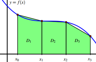
Figure 5.15: Estimating R b a f (x) dx using three subintervals and trapezoids, rather than rectangles, where a = x0 and b = x3.

Because both left and right endpoints are being used, we recognize within the trapezoidal approximation the use of both left and right Riemann sums. In particular, rearranging the expression for T3 by removing a factor of 1 2 , grouping the left endpoint evaluations of f , and grouping the right endpoint evaluations of f , we see that

\[T3 = 1 2 [( f (x0)4x + f (x1)4x + f (x2)4x) + ( f (x1)4x + f (x2)4x + f (x3)4x)] . (5.14)\]

At this point, we observe that two familiar sums have arisen. Since the left Riemann sum L3 is L3 = f (x0)4x + f (x1)4x + f (x2)4x, and the right Riemann sum is R3 = f (x1)4x + f (x2)4x + f (x3)4x, substituting L3 and R3 for the corresponding expressions in Equation 5.14, it follows that T3 = 1 2 [L3 + R3] . We have thus seen the main ideas behind a very important result: using trapezoids to estimate the (signed) area bounded by a curve is the same as averaging the estimates generated by using left and right endpoints. (The Trapezoid Rule) The trapezoidal approximation, Tn, of the definite integral R b a f (x) dx using n subintervals is given by the rule

\[Tn = 1 2 ( f (x0) + f (x1))4x + 1 2 ( f (x1) + f (x2))4x + · · · + 1 2 ( f (xn−1) + f (xn))4x. = Xn−1 i=0 1 2 ( f (xi) + f (xi+1))4x. \]

Moreover,

\[Tn = 1 2 [Ln + Rn] .\]

Exercise \(\PageIndex{2}\):

In this activity, we explore the relationships among the errors generated by left, right, midpoint, and trapezoid approximations to the definite integral R 2 1 1 x 2 dx

1. Use the First FTC to evaluate R 2 1 1 x 2 dx exactly.
2. Use appropriate computing technology to compute the following approximations for R 2 1 1 x 2 dx: T4, M4, T8, and M8.
3. Let the error of an approximation be the difference between the exact value of the definite integral and the resulting approximation. For instance, if we let ET,4 represent the error that results from using the trapezoid rule with 4 subintervals to estimate the integral, we have ET,4 = Z 2 1 1 x 2 dx − T4. Similarly, we compute the error of the midpoint rule approximation with 8 subintervals by the formula EM,8 = Z 2 1 1 x 2 dx − M8. Based on your work in (a) and (b) above, compute ET,4, ET,8, EM,4, EM,8.
4. Which rule consistently over-estimates the exact value of the definite integral? Which rule consistently under-estimates the definite integral?
5. What behavior(s) of the function f (x) = 1 x 2 lead to your observations in (d)? C

Comparing the Midpoint and Trapezoid Rules

We know from the definition of the definite integral of a continuous function f , that if we let n be large enough, we can make the value of any of the approximations Ln, Rn, and Mn as close as we’d like (in theory) to the exact value of R b a f (x) dx. Thus, it may be natural to wonder why we ever use any rule other than Ln or Rn (with a sufficiently large n value) to estimate a definite integral. One of the primary reasons is that as n → ∞, 4x = b−a n → 0, and thus in a Riemann sum calculation with a large n value, we end up multiplying by a number that is very close to zero. Doing so often generates roundoff error, as representing numbers close to zero accurately is a persistent challenge for computers. Hence, we are exploring ways by which we can estimate definite integrals to high levels of precision, but without having to use extremely large values of n. Paying close attention 324 5.6. NUMERICAL INTEGRATION to patterns in errors, such as those observed in Activity 5.15, is one way to begin to see some alternate approaches. To begin, we make a comparison of the errors in the Midpoint and Trapezoid rules from two different perspectives. First, consider a function of consistent concavity on a given interval, and picture approximating the area bounded on that interval by both the Midpoint and Trapezoid rules using a single subinterval. As seen in Figure 5.16, it

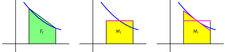
Figure 5.16: Estimating R b a f (x) dx using a single subinterval: at left, the trapezoid rule; in the middle, the midpoint rule; at right, a modified way to think about the midpoint rule.

is evident that whenever the function is concave up on an interval, the Trapezoid Rule with one subinterval, T1, will overestimate the exact value of the definite integral on that interval. Moreover, from a careful analysis of the line that bounds the top of the rectangle for the Midpoint Rule (shown in magenta), we see that if we rotate this line segment until it is tangent to the curve at the point on the curve used in the Midpoint Rule (as shown at right in Figure 5.16), the resulting trapezoid has the same area as M1, and this value is less than the exact value of the definite integral. Hence, when the function is concave up on the interval, M1 underestimates the integral’s true value. These observations extend easily to the situation where the function’s concavity remains consistent but we use higher values of n in the Midpoint and Trapezoid Rules. Hence, whenever f is concave up on [a, b], Tn will overestimate the value of R b a f (x) dx, while Mn will underestimate R b a f (x) dx. The reverse observations are true in the situation where f is concave down. Next, we compare the size of the errors between Mn and Tn. Again, we focus on M1 and T1 on an interval where the concavity of f is consistent. In Figure 5.17, where the error of the Trapezoid Rule is shaded in red, while the error of the Midpoint Rule is shaded lighter red, it is visually apparent that the error in the Trapezoid Rule is more significant.

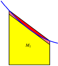
Figure 5.17: Comparing the error in estimating R b a f (x) dx using a single subinterval: in red, the error from the Trapezoid rule; in light red, the error from the Midpoint rule.

To see how much more significant, let’s consider two examples and some particular computations. If we let f (x) = 1 − x 2 and consider R 1 0 f (x) dx, we know by the First FTC that the exact value of the integral is Z 1 0 (1 − x 2 ) dx = x − x 3 3 1 0 = 2 3 . Using appropriate technology to compute M4, M8, T4, and T8, as well as the corresponding errors EM,4, EM,8, ET,4, and ET,8, as we did in Activity 5.15, we find the results summarized in Table 5.1. Note that in the table, we also include the approximations and their errors for the example R 2 1 1 x 2 dx from Activity 5.15.

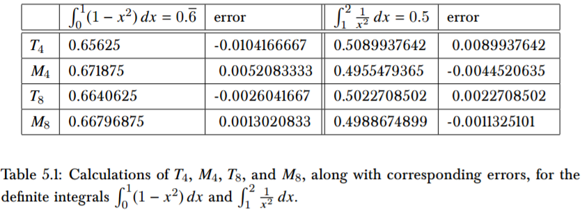
Table 5.1: Calculations of T4, M4, T8, and M8, along with corresponding errors, for the definite integrals R 1 0 (1 − x 2 ) dx and R 2 1 1 x 2 dx.

Recall that for a given function f and interval [a, b], ET,4 = R b a f (x) dx −T4 calculates the difference between the exact value of the definite integral and the approximation generated by the Trapezoid Rule with n = 4. If we look at not only ET,4, but also the other errors generated by using Tn and Mn with n = 4 and n = 8 in the two examples noted in Table 5.1, we see an evident pattern. Not only is the sign of the error (which measures whether the rule generates an over- or under-estimate) tied to the rule used and the function’s concavity, but the magnitude of the errors generated by Tn and Mn seems closely connected. In particular, the errors generated by the Midpoint Rule seem to be about half the size of those generated by the Trapezoid Rule. That is, we can observe in both examples that EM,4 ≈ −1 2 ET,4 and EM,8 ≈ −1 2 ET,8, which demonstrates a property of the Midpoint and Trapezoid Rules that turns out to hold in general: for a function of consistent concavity, the error in the Midpoint Rule has the opposite sign and approximately half the magnitude of the error of the Trapezoid Rule. Said symbolically, EM,n ≈ − 1 2 ET,n. This important relationship suggests a way to combine the Midpoint and Trapezoid Rules to create an even more accurate approximation to a definite integral. Simpson’s Rule When we first developed the Trapezoid Rule, we observed that it can equivalently be viewed as resulting from the average of the Left and Right Riemann sums: Tn = 1 2 (Ln + Rn). Whenever a function is always increasing or always decreasing on the interval [a, b], one of Ln and Rn will over-estimate the true value of R b a f (x) dx, while the other will under-estimate the integral. Said differently, the errors found in Ln and Rn will have opposite signs; thus, averaging Ln and Rn eliminates a considerable amount of the error present in the respective approximations. In a similar way, it makes sense to think about averaging Mn and Tn in order to generate a still more accurate approximation. At the same time, we’ve just observed that Mn is typically about twice as accurate as Tn. Thus, we instead choose to use the weighted average S2n = 2Mn + Tn 3 . (5.15) The rule for S2n giving by Equation 5.15 is usually known as Simpson’s Rule. 9 Note that we use “S2n” rather that “Sn” since the n points the Midpoint Rule uses are different from the n points the Trapezoid Rule uses, and thus Simpson’s Rule is using 2n points at which to evaluate the function. We build upon the results in Table 5.1 to see the approximations generated by Simpson’s Rule. In particular, in Table 5.2, we include all of the results in 9Thomas Simpson was an 18th century mathematician; his idea was to extend the Trapezoid rule, but rather than using straight lines to build trapezoids, to use quadratic functions to build regions whose area was bounded by parabolas (whose areas he could find exactly). Simpson’s Rule is often developed from the more sophisticated perspective of using interpolation by quadratic functions. 5.6. NUMERICAL INTEGRATION 327 Table 5.1, but include additional results for S8 = 2M4+T4 3 and S16 = 2M8+T8 3 . R 1 0 (1 − x 2 ) dx = 0.6

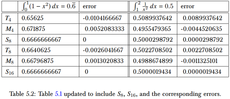
Table 5.2: Table 5.1 updated to include S8, S16, and the corresponding errors.

The results seen in Table 5.2 are striking. If we consider the S16 approximation of R 2 1 1 x 2 dx, the error is only ES,16 = 0.0000019434. By contrast, L8 = 0.5491458502, so the error of that estimate is EL,8 = −0.0491458502. Moreover, we observe that generating the approximations for Simpson’s Rule is almost no additional work: once we have Ln, Rn, and Mn for a given value of n, it is a simple exercise to generate Tn, and from there to calculate S2n. Finally, note that the error in the Simpson’s Rule approximations of R 1 0 (1 − x 2 ) dx is zero!10 These rules are not only useful for approximating definite integrals such as R 1 0 e −x 2 dx, for which we cannot find an elementary antiderivative of e −x 2 , but also for approximating definite integrals in the setting where we are given a function through a table of data.

Exercise \(\PageIndex{3}\):

A car traveling along a straight road is braking and its velocity is measured at several different points in time, as given in the following table. Assume that v is continuous, always decreasing, and always decreasing at a decreasing rate, as is suggested by the data.

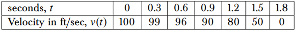
1. Plot the given data on the set of axes provided in Figure 5.18 with time on the horizontal axis and the velocity on the vertical axis.
2. What definite integral will give you the exact distance the car traveled on [0, 1.8]? 10Similar to how the Midpoint and Trapezoid approximations are exact for linear functions, Simpson’s Rule approximations are exact for quadratic and cubic functions. See additional discussion on this issue later in the section and in the exercises.
3. Estimate the total distance traveled on [0, 1.8] by computing L3, R3, and T3. Which of these under-estimates the true distance traveled?
4. Estimate the total distance traveled on [0, 1.8] by computing M3. Is this an over- or under-estimate? Why?
5. Using your results from (c) and (d), improve your estimate further by using Simpson’s Rule.
6. What is your best estimate of the average velocity of the car on [0, 1.8]? Why? What are the units on this quantity?

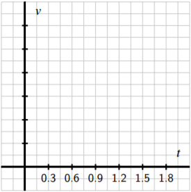
Figure 5.18: Axes for plotting the data in Activity 5.16.

Overall observations regarding Ln, Rn, Tn, Mn, and S2n. As we conclude our discussion of numerical approximation of definite integrals, it is important to summarize general trends in how the various rules over- or under-estimate the true value of a definite integral, and by how much. To revisit some past observations and see some new ones, we consider the following activity.

Activity \(\PageIndex{4}\):

Consider the functions f (x) = 2 − x 2 , g(x) = 2 − x 3 , and h(x) = 2 − x 4 , all on the interval [0, 1]. For each of the questions that require a numerical answer in what follows, write your answer exactly in fraction form.

1. On the three sets of axes provided in Figure 5.19, sketch a graph of each function on the interval [0, 1], and compute L1 and R1 for each. What do you observe? 5.6. NUMERICAL INTEGRATION 329
2. Compute M1 for each function to approximate R 1 0 f (x) dx, R 1 0 g(x) dx, and R 1 0 h(x) dx, respectively.
3. Compute T1 for each of the three functions, and hence compute S1 for each of the three functions.
4. Evaluate each of the integrals R 1 0 f (x) dx, R 1 0 g(x) dx, and R 1 0 h(x) dx exactly using the First FTC.
5. For each of the three functions f , g, and h, compare the results of L1, R1, M1, T1, and S2 to the true value of the corresponding definite integral. What patterns do you observe?

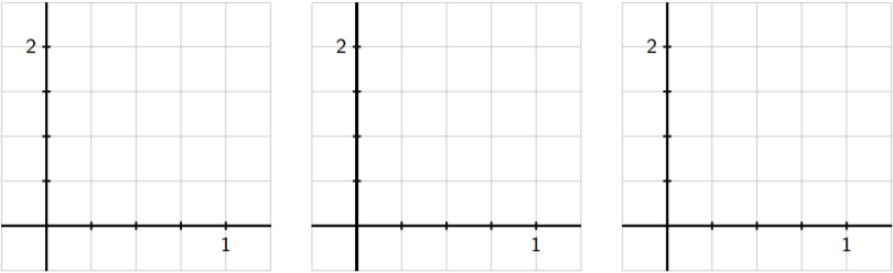
Figure 5.19: Axes for plotting the functions in Activity 5.17.

The results seen in the examples in Activity 5.17 generalize nicely. For instance, for any function f that is decreasing on [a, b], Ln will over-estimate the exact value of R b a f (x) dx, and for any function f that is concave down on [a, b], Mn will over-estimate the exact value of the integral. An excellent exercise is to write a collection of scenarios of possible function behavior, and then categorize whether each of Ln, Rn, Tn, and Mn is an over- or under-estimate. Finally, we make two important notes about Simpson’s Rule. When T. Simpson first developed this rule, his idea was to replace the function f on a given interval with a quadratic function that shared three values with the function f . In so doing, he guaranteed that this new approximation rule would be exact for the definite integral of any quadratic polynomial. In one of the pleasant surprises of numerical analysis, it turns out that even though it was designed to be exact for quadratic polynomials, Simpson’s Rule is exact for any cubic polynomial: that is, if we are interested in an integral such as R 5 2 (5x 3 −2x 2 +7x −4) dx, S2n will always be exact, regardless of the value of n. This is just one more piece of evidence that shows how effective Simpson’s Rule is as an approximation tool for estimating definite integrals.11

Summary

In this section, we encountered the following important ideas:

• For a definite integral such as R 1 0 e −x 2 dx when we cannot use the First Fundamental Theorem of Calculus because the integrand lacks an elementary algebraic antiderivative, we can estimate the integral’s value by using a sequence of Riemann sum approximations. Typically, we start by computing Ln, Rn, and Mn for one or more chosen values of n.
• The Trapezoid Rule, which estimates R b a f (x) dx by using trapezoids, rather than rectangles, can also be viewed as the average of Left and Right Riemann sums. That is, Tn = 1 2 (Ln + Rn).
• The Midpoint Rule is typically twice as accurate as the Trapezoid Rule, and the signs of the respective errors of these rules are opposites. Hence, by taking the weighted average Sn = 2Mn+Tn 3 , we can build a much more accurate approximation to R b a f (x) dx by using approximations we have already computed. The rule for Sn is known as Simpson’s Rule, which can also be developed by approximating a given continuous function with pieces of quadratic polynomials.

Contributors and Attributions

• Matt Boelkins (Grand Valley State University), David Austin (Grand Valley State University), Steve Schlicker (Grand Valley State University)