1.9: Answers to exercises

Answer to the question of how to find the R command if you know only what it should do (e.g., “anova”). In order to find this from within R, you may go in several ways. First is to use double question marks command ??:

Code \(\PageIndex{1}\) (R):

??anova

(Output might be long because it includes all installed packages. Pay attention to rows started with “base” and “stats”.)

Similar result might be achieved if you start the interactive (Web browser-based) help with help.start() and then enter “anova” into the search box.

Second, even simpler way, is to use apropos():

Code \(\PageIndex{2}\) (R):

apropos("anova")

Sometimes, nothing helps:

Code \(\PageIndex{3}\) (R):

??clusterization
apropos("clusterization")

Then start to search in the Internet. It might be done from within R:

Code \(\PageIndex{4}\) (R):

RSiteSearch("clusterization")

In the Web browser, you should see the new tab (or window) with the query results.

If nothing helps, as the R community. Command help.request() will guide you through posting sequence.

Answer to the plot question (Figure 2.8.4):

Code \(\PageIndex{5}\) (R):

plot(1:20, col="green", xlab="", ylab="")
points(20:1, pch=0)

(Here empty xlab and ylab were used to remove axes labels. Note that pch=0 is the rectangle.)

Instead of col="green", one can use col=3. See below palette() command to understand how it works. To know all color names, type colors(). Argument col could also have multiple values. Check what happen if you supply, saying, col=1:3 (pay attention to the very last dots).

To know available point types, run example(points) and skip several plots to see the table of points; or simply look on Figure A.1.1 in this book (and read comments how it was made).

Answer to the question about eggs. First, let us load the data file. To use read.table() command, we need to know file structure. To know the structure, (1) we need to look on this file from R with url.show() (or without R, in the Internet browser), and also (2) to look on the companion file, eggs_c.txt.

From (1) and (2), we conclude that file has three nameless columns from which we will need first and second (egg length and width in mm, respectively). Columns are separated with large space, most likely the Tab symbol. Now we can run read.table():

Code \(\PageIndex{6}\) (R):

eggs <- read.table("data/eggs.txt")

Next step is always to check the structure of new object:

Code \(\PageIndex{7}\) (R):

eggs <- read.table("data/eggs.txt")
str(eggs)

It is also the good idea to look on first rows of data:

Code \(\PageIndex{8}\) (R):

eggs <- read.table("data/eggs.txt")
head(eggs)

Our first and second variables received names V1 (length) and V2 (width). Now we need to plot variables to see possible relation. The best plot in that case is a scatterplot, and to make scatterplot in R, we simply use plot() command:

Code \(\PageIndex{9}\) (R):

plot(V2 ~ V1, data=eggs, xlab="Length, mm", ylab="Width, mm", pch=21, bg="grey")

(Command plot(y ~ x) uses Rformula interface. It is almost the same as plot(x, y)\(^{[1]}\); but note the different order in arguments.)

Resulted “cloud” is definitely elongated and slanted as it should be in case of dependence. What would make this more clear, is some kind of the “average” line showing the direction of the relation. As usual, there are several possibilities in R (Figure \(\PageIndex{1}\)):

Code \(\PageIndex{10}\) (R):

abline(line(eggs$V1, eggs$V2), lty=2, lwd=1.5)
lines(loess.smooth(eggs$V1, eggs$V2), col=2, lty=2, lwd=1.5)
legend("topleft", lty=2, col=1:2, lwd=1.5, legend=c("Tukey's median-median line", "LOESS curve"))

(Note use of line(), lines() and abline()—all three are really different commands. lines() and abline() are low-level graphic commands which add line(s) to the existing plot. First uses coordinates while the second uses coefficients. line() and loess.smooth() do not draw, they calculate numbers to use with drawing commands. To see this in more details, run help() for every command.)

First line() approach uses John Tukey’s algorithm based on medians (see below) whereas loess.smooth() uses more complicated non-linear LOESS (LOcally wEighted Scatterplot Smoothing) which estimates the overall shape of the curve\(^{[2]}\). Both are approximate but robust, exactly what we need to answer the question. Yes, there is a dependence between egg maximal width and egg maximal length.

There is one problem though. Look on the Figure \(\PageIndex{1}\): many “eggs” are overlaid with other points which have exact same location, and it is not easy to see how many data belong to one point. We will try to access this in next chapter.

Answer to the R script question. It is enough to create (with any text editor) the text file and name it, for example, my_script1.r. Inside, type the following:

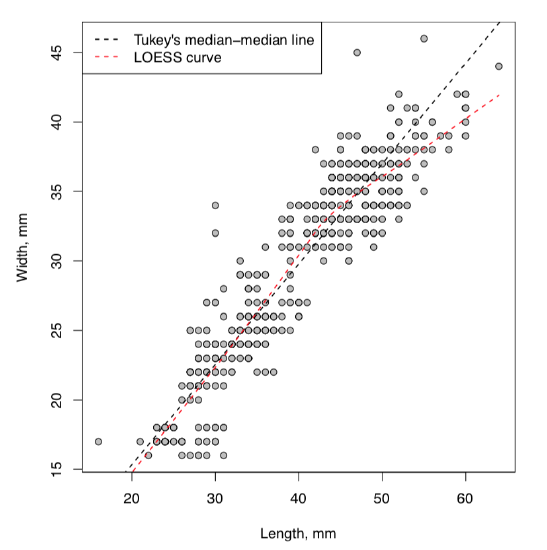Figure \(\PageIndex{1}\) Cloud of eggs: scatterplot.

pdf("my_plot1.pdf")
plot(1:20)
dev.off()

Create the subdirectory test and copy your script there. Then close R as usual, open it again, direct it (through the menu or with setwd() command) to make the test subdirectory the working directory, and run:

Code \(\PageIndex{11}\) (R):

source("my_script1.r", echo=TRUE)

If everything is correct, then the file my_plot1.pdf will appear in the test directory. Please do not forget to check it: open it with your PDF viewer. If anything went wrong, it is recommended to delete directory test along with all content, modify the master copy of script and repeat the cycle again, until results become satisfactory.

References

1. In the case of our eggs data frame, the command of second style would be plot(eggs[, 1:2]) or plot(eggs$V1, eggs$V2),seemoreexplanationsinthenextchapter.

2. Another variant is to use high-level scatter.smooth() function which replaces plot(). Third alternative is a cubic smoother smooth.spline() which calculates numbers to use with lines().