
part0001
- Page ID
- 24587
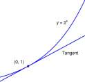
A tangent to a graph is a polynomial of degree one “close to” the graph. The graph of F(x) = 2 X and the tangent
P x {x) = 1 + 0.69315x – 1 < x < 2
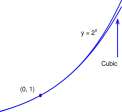
at (0,1) are shown in Figure 2.4(a). The graph of the cubic polynomial
P 3 ( x ) = 1 + 0.69315 x + 0.24023 x 2 + 0.05550 x 3 -l<x<2
shown in Figure 2.4(b) is even closer to the graph of F(x) = 2 X . These graphs are hardly distinguishable on — 1 < x < 1 and only clearly separate at about x = 1.5. The function F(x) = 2 X is difficult to evaluate (without a calculator) except at integer values of x, but /^(x) can be evaluated with just multiplication and addition. For x = 0.5, F(0.5) = 2 0 5 = y/2 = 1.41421 and Ps(0.5) = 1.41375. The relative error in using Ps(0.5) as an approximation to a/2 is
Relative Error
P 3 (0.5)-F(0.5)
F(0.5)
The relative error is less than 0.04 percent.
1.41375 – 1.41421
1.41421
0.00033
A
Tangent
B
Cubic
Figure 2.4: A. Graph of y = 2 X and its tangent at (0,1), P\{x) = 1 + 0.69315a;. B. Graph of y = 2 2 and the cubic, P 3 (x) = 1 + 0.69315 x + 0.24023 x 2 + 0.05550 x 3 .
The tangent P±(x) is a good approximation to F(x) = 2 X near the point of tangency (0,1) and the cubic polynomial Ps(x) is an even better approximation. The coefficients 0.69135, 0.24023, and 0.05550 are presented here as Lightning Bolts Out of the Blue. A well defined procedure for selecting the coefficients is defined in Chapter 12.
Explore 2.4.1 Find the relative error in using the tangent approximation, Pi(0.5) = 1 + 0.69315 x 0.5 as an approximation to P(0.5) = 2 a5 . ■
Example 2.4.1 Problem. Show that polynomials are linear in their coefficients. This means that
• The sum of two polynomials is obtained by adding ‘corresponding’ coefficients (add the constant terms, add the coefficients of x, add the coefficients of x 2 , ■ ■ ■ ).
• The product of a constant, K, and a polynomial, P(x), is the polynomial whose coefficients are the coefficients of P(x) each multiplied by K.
Consider the following.
Let P(x) = 7-3x + 5x 2 , and Q(x) = -2 + Ax – x 2 + Qx 3 .
P(x) + Q(x) = (7 -3x + 5x 2 ) + {-2 + 4x – x 2 + 6x 3
= (7-2) + (-3 + 4)x + (5-l)a; 2 + (0 + 6)x 3 = 5 + x + 4x 2 + 6x 3
Thus P(x) + Q(x) is simply the polynomial obtained by adding corresponding coefficients in P(x) and Q(x). Furthermore,
13-P(x) = 13(7-3x + 5x 2 ) = 13-7-13-3a; + 13-5a; 2 = 91-39a; + 65a: 2 .
Thus 13 ■ P(x) is simply the polynomial obtained by multiplying each coefficient of P(x) by 13. On the other hand, for
P(x) = 5 sin 3x, Q(x) = 6 sin Ax,
P(x) + Q(x) = 5 sin 3a;+ 6 sin 4x ^ (5 + 6) sin( (3 + 4) x ) = 11 sin 7x. The sine functions are not linear in their coefficients.
Exercises for Section 2.4 Polynomial functions. Exercise 2.4.1 Technology. Let F(x) = y/x. The polynomials
P 2 (x) = l + -x–x and P 3{x ) = – + -x- — x + — x*
closely approximate F near the point (4,2) of F.
a. Draw the graphs of F and P 2 on the range 1 < x < 8.
b. Compute the relative error in ^2(2) as an approximation to F{2) = \/2.
c. Draw the graphs of F and ^3(0;) on the range 1 < x < 8.
d. Compute the relative error in ^3(2) as an approximation to F{2) = \/2.
CHAPTER 2. DESCRIPTIONS OF BIOLOGICAL PATTERNS
70
A
B
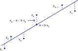
Figure 2.5: A. Least squares fit of a line to data. B. Least squares fit of a parabola to data.
Exercise 2.4.2 Technology. Let F(x) = {/x. The polynomials
P 2 {x) = – + -x-^x 2 and P 3 (x) = P 2 (x) + — (x – l) 3 closely approximate F near the point (1,1) of F.
a. Draw the graphs of F and P% on the range 0 < x < 3.
b. Compute the relative error in P2(2) as an approximation to F{2) = \[2.
c. Draw the graphs of F and P3 on the range 1 < x < 3.
d. Compute the relative error in P%{2) as an approximation to F{2) = \/2.
2.5 Least squares fit of polynomials to data
Polynomials and especially linear functions are often ‘fit’ to data as a means of obtaining a brief and concise description of the data. The most common and widely used method is the method of least squares. To fit a line to a data set, (xi,yi), (x 2 ,1/2), • • • (x n , y n ), one selects a and b that minimizes
n
X; (y k -a-bx k f (2.2) k=i
The geometry of this equation is illustrated in Figure 2.5. The goal is to select a and b so that the sum of the squares of the lengths of the dashed lines is as small as possible. We show in in Example 13.2.2 that the optimum values of a and b satisfy
an + &Efc=i %k = Efc=i Vk
(2.3)
CHAPTER 2. DESCRIPTIONS OF BIOLOGICAL PATTERNS
Table 2.2: Relation between temperature and frequency of cricket chirps.
Temperature °F Chirps per
Minute 109 136 160 87 103 102 108 154 144 150
The solution to these equations is
a =
Y. x lY.Vk – I 2 x k) [Y, x kVk
k=l k=l \fc=l / \fc=l /
A
k=l \fc=l / Vfc=l /
A
\ 2
n in
A = nJ2 %l ~ (J2 x k)
k=l \k=l I
Example 2.5.1 If we use these equations to fit a line to the cricket data of Example 1.10.1 showing a relation between temperature and cricket chirp frequency, we get
y = 4.5008a; – 192.008, close to the line y = 4.5x – 192
that we ‘fit by eye’ using the two points, (65,100) and (75,145).
Explore 2.5.1 Technology. Your calculator or computer will hide all of the arithmetic of Equations 2.4 and give you the answer. The overall procedure is:
1. Load the data. [Two lists, X and Y, say].
2. Compute the coefficients of a first degree polynomial close to the data and store them in P.
3. Specify X coordinates and compute corresponding Y coordinates for the polynomial.
4. Plot the original data and the computed polynomial.
A MATLAB program to do this is:
close all;clc;clear
X=[67 73 78 61 66 66 67 77 74 76] ;
Y=[109 136 160 87 103 102 108 154 144 150];
P=polyfit(X,Y,l)
PX=[60:0.1:80];
PY=polyval(P,PX);
plot(X,Y,’+’,’linewidth’,2); hold(‘on’); plot(PX,PY,’linewidth’,2)
Table 2.3: A tube is filled with water and a hole is opened at the bottom of the tube. Relation between height of water remaining in the tube and time.
Time sec 0 5 10 15 20 25 30 35 40 45 50 55 60
Height cm 85 73 63 54 45 36 29 22 17 12 7 4 2
To fit a parabola to a data set, (xi,yi), (£2,2/2), • • • (x n ,y n ), one selects a, b and c that minimizes
n
(y k -a-bx k -cx 2 k ) 2 (2.5)
k=i
The geometry of this equation is illustrated in Figure 2.5B. The goal is to select a, b and c so that the sum of the squares of the lengths of the dashed lines is as small as possible. The optimum values of a, b, and c satisfy (Exercise 14.2.4)
There is a methodical procedure for solving three linear equations three variables using pencil and paper. For now it is best to rely on your calculator or computer.
Explore 2.5.2 Technology. Fit a parabola to the water draining from a tube data of Figure 1.25 reproduced in Table 2.3.
The procedure will be almost identical to that of Explore 2.5.1. The difference is that in step 2 you will compute the coefficients of a second degree polynomial. The line P=polyf it (X,Y, 1) will be changed to P=polyf it (X,Y,2) . In the program, of course, the data will be different and the PX-values for the polynomial will be adjusted to the data. ■
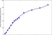
Example 2.5.2 A graph of the polio data from Example 2.2.1 showing the percent of U.S. population that had antibodies to the polio virus in 1955 is shown in Figure 2.6. Also shown is a graph of the fourth degree polynomial
P 4 (x) = -4.13 + 7.57a; – 0.136a; 2 – 0.00621a; 3 + 0.000201a; 4
The polynomial that ‘fit’ the polio data using a MATLAB program similar to that described in Explore 2.5.1 and discussed in Explore 2.5.2 The technology selects the coefficients, -4.14, 7.57, • • • so that the sum of the squares of the distances from the polynomial to the data is as small as possible. ■
CHAPTER 2. DESCRIPTIONS OF BIOLOGICAL PATTERNS
73
0 10 20 30
Figure 2.6: A fourth-degree polynomial fit to data for percent of people in 1955 who had antibodies to the polio virus as a function of age. Data read from Anderson and May, Vaccination and herd immunity to infectious diseases, Nature 318 1985, pp 323-9, Figure 2f.
Exercises for Section 2.5, Least squares fit of polynomials to data.
Exercise 2.5.1 Use Equations 2.3 to find the linear function that is the least squares fit to the data:
(-2,5) (3,12)
Exercise 2.5.2 Use Equations 2.6 to find the quadratic function that is the least squares fit to the data:
(-2,5) (3,12) (10,0)
Exercise 2.5.3 Technology Shown in the Table 2.4 are the densities of water at temperatures from 0 to 100 °C Use your calculator or computer to fit a cubic polynomial to the data. See Explore 2.5.1 and Explore 2.5.2. Compare the graphs of the data and of the cubic.
Table 2.4: The density of water at various temperatures Source: Robert C. Weast, Melvin J. Astle, and William H. Beyer, CRC Handbook of Chemistry and Physics, 68th Edition, 1988, CRC Press, Boca Raton, FL, p F-10.
CHAPTER 2. DESCRIPTIONS OF BIOLOGICAL PATTERNS
74
2.6 New functions from old.
It is often important to recognize that a function of interest is made up of component parts — other functions that are combined to make up the function of central interest. Researchers monitoring natural populations (deer, for example) partition the dynamics into the algebraic sum of births, deaths, and harvest. Researchers monitoring annual grain production in the United States decompose the production into the product of the number of acres planted and yield per acre.
Total Corn Production = Acres Planted to Corn x Yield per Acre Pit) = A(t) x Y(t)
Factors that influence A(t), the number of acres planted (government programs, projected corn price, alternate cropping opportunities, for example) are qualitatively different from the factors that influence Y(t), yield per acre (corn genetics, tillage practices, and weather).
2.6.1 Arithmetic combinations of functions.
A common mathematical strategy is “divide and conquer” — partition your problem into smaller problems, each of which you can solve. Accordingly it is helpful to recognize that a function is composed of component parts. Recognizing that a function is the sum, difference, product, or quotient of two functions is relatively simple.
For example F(t) = 2* + 1 2 is the sum of an exponential function, E(t) = 2* and a quadratic function, S(t) = t 2 . Which of the two functions dominates (contributes most to the value of F) for t < 0? For t > 0 (careful here, the graphs are incomplete). Shown in Figure 2.7 are the graphs of E and S.
Next in Figure 2.8 are the graphs of
E
E + S, E-S, Ex S, and —
o
but not necessarily in that order. Which graph depicts which of the combinations of S and El
CHAPTER 2.
DESCRIPTIONS OF BIOLOGICAL PATTERNS
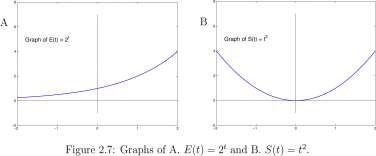
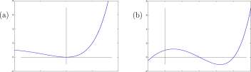
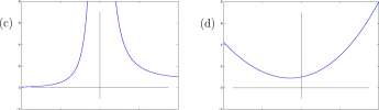
Figure 2.8: Graphs of the sum, difference, product, and quotient of E(t) = 2* and S(t) = t 2 .
Note first that the domains of E and S are all numbers, so that the domains of E + S, E — S, and E x S are also all numbers. However, the domain of E/S excludes 0 because S(0) = 0 and E(0)/S(0) = 1/0 is meaningless.
The graph in Figure 2.8(c) appears to not have a point on the y-axis, and that is a good candidate for E/S. E(t) and S(t) are never negative, and the sum, product, and quotient of non-negative numbers are all non-negative. However, the graph in Figure 2.8(b) has some points below the and that is a good candidate for E — S.
The product, E x S is interesting for t < 0. The graph of E = 2* is asymptotic to the negative t-axis; as t progresses from -1 to -2 to -3 to • • •, E(t) is 2″ 1 = 0.5, 2″ 2 = 0.25, 2″ 3 = 0.125, • • • and gets close to zero. But S(t) = t 2 is (—l) 2 = 1, (—2) 2 = 3, (—3) 2 = 9, • • • gets very large. What does the product do?
CHAPTER 2. DESCRIPTIONS OF BIOLOGICAL PATTERNS
76
2.6.2 The inverse of a function.
Suppose you have a travel itinerary as shown in Table 2.5. If your traveling companion asks,
Table 2.5: Itinerary for (brief) European trip.
Day June 1 June 2 June 3 June 4 June 5 June 6 June 7 City London London London Brussels Paris Paris Paris
“What day were we in Brussels?”, you may read the itinerary ‘backward’ and respond that you were in Brussels on June 4. On the other hand, if your companion asks, “I cashed a check in Paris, what day was it?”, you may have difficulty in giving an answer.
An itinerary is a function that specifies that on day, x, you will be in location, y. You have inverted the itinerary and reasoned that the for the city Brussels, the day was June 4. Because you were in Paris June 5-7, you can not specify the day that the check was cashed.
Charles Darwin exercised an inverse in an astounding way. In his book, On the Various Contrivances by which British and Foreign Orchids are Fertilised by Insects he stated that the angraecoids were pollinated by specific insects. He noted that A. sesquipedale in Madagascar had nectaries eleven and a half inches long with only the lower one and one-half inch filled with nectar. He suggested the existence of a ‘huge moth, with a wonderfully long proboscis’ and noted that if the moth ‘were to become extinct in Madagascar, assuredly the Angraecum would become extinct.’ Forty one years later Xanthopan morgani praedicta was found in tropical Africa with a proboscis of ten inches.
Such inverted reasoning occurs often.
Explore 2.6.1 Answer each of the following by examining the inverse of the function described.
a. Rate of heart beat increases with level of exertion; heart is beating at 165 beats per minute; is the level of exertion high or low? You may want to visit en.wikipedia.org/wiki/Heart_rate.
b. Resting blood pressure goes up with artery blockage; resting blood pressure is 110 (systolic) ‘over’ 70 (diastolic); is the level of artery blockage high or low? The answer can be found in en.wikipedia.org/wiki/Blood_Pressure.
c. Diseases have symptoms; a child is observed with a rash over her body. Is the disease chicken pox?
The child with a rash in Example c. illustrates again an ambiguity often encountered with inversion of a function; the child may in fact have measles and not chicken pox. The inverse information may be multivalued and therefore not a function. Nevertheless, the doctor may make a diagnosis as the most probable disease, given the observed symptoms. She may be influenced by facts such as
• Blood analysis has demonstrated that five other children in her clinic have had chicken pox that week and,
• Because of measles immunization, measles is very rare.
CHAPTER 2. DESCRIPTIONS OF BIOLOGICAL PATTERNS
77
It may be that she can actually distinguish chicken pox rash from measles rash, in which case the ambiguity disappears.
The definition of the inverse of a function is most easily made in terms of the ordered pair definition of a function. Recall that a function is a collection of ordered number pairs, no two of which have the same first term.
Definition 2.6.2 Inverse of a Function. A function F is invertible if no two ordered pairs of F have the same second number. The inverse of an invertible function, F, is the function G to which the ordered pair (x,y) belongs if and only if (y,x) is an ordered pair of F. The function, G, is often denoted by F1 .
Explore 2.6.2 Do This. Suppose G is the inverse of an invertible function F. What is the inverse ofG? ■
Table 2.6: Of the two itineraries shown below, the one on the left is invertible.
The notation F^ 1 for the inverse of a function F is distinct from the use of _1 as an exponent meaning division, as in 2~ 1 = \. In this context, F^ 1 does not mean j?, even though students have good reason to think so from previous use of the symbol, -1 . The TI-86 calculator (and others) have keys marked sin -1 and x -1 . In the first case, the _1 signals the inverse function, arcsinx, in the second case the _1 signals reciprocal, \jx. Given our desire for uniqueness of definition and notation, the ambiguity is unfortunate and a bit ironic. There is some recovery, however. You will see later that the composition of functions has an algebra somewhat like ‘multiplication’ and that ‘multiplying’ by an inverse of a function F has some similarity to ‘dividing’ by F. At this stage, however, the only advice we have is to interpret h” 1 as ‘divide by K if h is a number and as ‘inverse of K if h is a function or a graph.
The graph of a function easily reveals whether it is invertible. Remember that the graph of a function is a simple graph, meaning that no vertical line contains two points of the graph.
Definition 2.6.3 Invertible graph. An invertible simple graph is a simple graph for which no horizontal line contains two points. A simple graph is invertible if and only if it is the graph of an invertible function.
CHAPTER 2. DESCRIPTIONS OF BIOLOGICAL PATTERNS
78
The simple graph G in Figure 2.9(a) has two points on the same horizontal line. The points have the same ^/-coordinate, y±, and thus the function defining G has two ordered pairs, (xx,yi) and (x2,yi) with the same second term. The function is not invertible. The same simple graph G does contain a simple graph that is invertible, as shown as the solid curve in Figure 2.9(b), and it is maximal in the sense that if any additional point of the graph of G is added to it, the resulting graph is not invertible.
a.
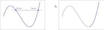
Figure 2.9: Graph of a function that is not invertible.
Explore 2.6.3 Find another simple graph contained in the graph G of Figure 2.9(a) that is invertible. Is your graph maximal? Is there a simple graph contained in G other than that shown in Figure 2.9 that is invertible and maximal? ■
Example 2.6.1 Shown in Figure 2.10 is the graph of an invertible function, F, as a solid line and the graph of F~ x as a dashed line. Tables of seven ordered pairs of F and seven ordered pairs of F are given. Corresponding to the point, P (3.0,1.4) of F is the point, Q (1.4,3.0) of The line y = x is the perpendicular bisector of the interval, PQ. Observe that the domain of F~ x is the range of F, and the range of F^ 1 is the domain of F. m ■
The preceding example lends support for the following observation.
The graph of the inverse of F is the reflection of the graph of F about the diagonal line, y = x.
The reflection of G with respect to the diagonal line, y = x consists of the points Q such that either Q is a point of G on the diagonal line, or there is a point P of G such that the diagonal line is the perpendicular bisector of the interval PQ.
The concept of the inverse of a function makes it easier to understand logarithms. Shown in Table 2.7 are some ordered pairs of the exponential function, F{x) = 10 x and some ordered pairs of the logarithm function G(x) = log 10 (x). The logarithm function is simply the inverse of the exponential function.
CHAPTER 2. DESCRIPTIONS OF BIOLOGICAL PATTERNS
79
4.5 –
(1.4,3.0)
0.5 –
0 0.5 1 1.5 2 2.5 3 3.5 4 4.5 5
Figure 2.10: Graph of a function F (solid line) and its inverse F _1 (dashed line) and tables of data for F and F~ l .
Table 2.7: Partial data for the function F(x) = 10 x and its inverse G(x) = log 10 (x).
The function F(x) = x 2 is not invertible. In Figure 2.11 both (-2,4) and (2,4) are points of the graph of F so that the horizontal line y = 4 contains two points of the graph of F. However, the function S defined by
S(x) =x 2 for x > 0 (2.7)
is invertible and its inverse is
S-Hx) = Jx~.
2.6.3 Finding the equation of the inverse of a function.
There is a straightforward means of computing the equation of the inverse of a function from the equation of the function. The inverse function reverses the role of the independent and dependent variables. The independent variable for the function is the dependent variable for the inverse function. To compute the equation for the inverse function, it is common to interchange the symbols for the dependent and independent variables.
Example 2.6.2 To compute the equation for the inverse of the function S,
CHAPTER 2. DESCRIPTIONS OF BIOLOGICAL PATTERNS
80
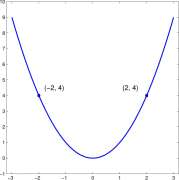
Figure 2.11: Graph of F(x) = x 2 ; (-2,4) and (2,4) are both points of the graph indicating that F is not invert ible.
let the equation for S be written as
Then interchange y and x to obtain
and solve for y.
y = x 2 for x > 0
x = y 2 for y > 0
x = y 2 for y > 0 y 2 = x for y > 0
.r –
2 i i ?/ 2 = x 2
i
y = X 2
Therefore
S 1 (x) = for x > 0
Example 2.6.3 The graph of function F(x) = 2x 2 — 6x + 3/2 shown in Figure 2.12 has two invertible portions, the left branch and the right branch. We compute the inverse of each of them. Let y = 2x 2 — 6x + 5/2, exchange symbols x = 2y 2 — 6y + 5/2, and solve for y. We use the
CHAPTER 2. DESCRIPTIONS OF BIOLOGICAL PATTERNS
-5 1 1 1 1 1 1 1 1 1
-3 -2 -1 0 1 2 3 4 5 6
Figure 2.12: Graph of F(x) = 2x 2 — 6x + 3/2 showing the left branch as dashed line and right branch as solid line.
steps of ‘completing the square’ that are used to obtain the quadratic formula.
x = 2y 2 -6y + 5/2
= 2(y 2 -3x + 9/4) – 9/2 + 5/2
= 2( 2 /-3/2) 2 -2
(y-m 2 = ^
,-3/2 = ,/^ + 2 or
1 \i ~2 ^ Right branch inverse.
3 X + 2 2 ~
Left branch inverse.
Exercises for Section 2.6 New functions from old. Exercise 2.6.1 In Figure 2.8 identify the graphs of E + S and E x S.
Exercise 2.6.2 Three examples of biological functions and questions of inverse are described Explore 2.6.1. Identify two more functions and related inverse questions.
CHAPTER 2. DESCRIPTIONS OF BIOLOGICAL PATTERNS
82
Exercise 2.6.3 The genetic code appears in Figure 2.3. It occasionally occurs that the amino acid sequence of a protein is known, and one wishes to know the DNA sequence that coded for it. That the genetic code is not invertible is illustrated by the following problem.
Find two DNA sequences that code for the amino acid sequence KYLEF. (Note: K = Lys = lysine, Y = Tyr = tyrosine, L = Leu = leucine, E = Glu = glutamic acid, F = Phe = phenylalanine. The sequence KYLEF occurs in sperm whale myoglobin.)
Exercise 2.6.4 Which of the following functions are invertible?
a. The distance a DNA molecule will migrate during agarose gel electrophoresis as a function of the molecular weight of the molecule, for domain: lkb < Number of bases < 20kb.
b. The density of water as a function of temperature.
c. Day length as a function of elevation of the sun above the horizon (at, say, 40 degrees North latitude).
d. Day length as a function of day of the year.
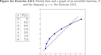
Exercise 2.6.5 Shown in Figure Ex. 2.6.5 is the graph of a function, F. Some ordered pairs of the function are listed in the table and plotted as filled circles. What are the corresponding ordered pairs of F~ l l Plot those points and draw the graph of
Exercise 2.6.6 Shown in Figure Ex. 2.6.6 is the graph of F(x) = 2 X . (-2,1/4), (0,1), and (2,4) are ordered pairs of F. What are the corresponding ordered pairs of F~ l l Plot those points and draw the graph of
CHAPTER 2. DESCRIPTIONS OF BIOLOGICAL PATTERNS
83
Figure for Exercise 2.6.6 Graph of F(x) = 2 X and the diagonal, y = x. See Exercise 2.6.6

(-2,1/4)
(2,4)
-10 12 3
Exercise 2.6.7 In Subsection 2.2.2 Simple Graphs and Figure 2.2 it is observed that the circle is not a simple graph but contained several simple graphs that were ‘as large as possible’, meaning that if another point of the circle were added to them they would not be simple graphs. Neither of the examples in Figure 2.2 is invertible. Does the circle contain a simple graph that is as large as possible and that is an invertible simple graph?
Exercise 2.6.8 Shown in Figure Ex. 2.6.8 is a graph of a function, F. Make a table of F and F~ l and plot the points of the inverse. Let G be F~ l . Make a table of G _1 and plot the points of G~ x .
Figure for Exercise 2.6.8 Graph of a function F. See Exercise 2.6.8. F1 = G
F
G1
Exercise 2.6.9 Is there an invertible function whose domain is the set of positive numbers and whose range is the set of non-negative numbers?
CHAPTER 2. DESCRIPTIONS OF BIOLOGICAL PATTERNS
84
Exercise 2.6.10 Incredible! Find the inverse of the function, F, defined by
F(x) = x1
Hint: Look at its graph.
Exercise 2.6.11 Answer the question in Explore 2.6.2, Suppose G is the inverse of an invertible function F. What is the inverse of G?
Exercise 2.6.12 Find equations for the inverses of the functions defined by
10-* 2 for x > for z > 1
Hint for (g): Let y = 2 * 2 2 -, interchange x and y so that x = 2V 2 2 , then substitute z = 2 y and solve for z in terms of x. Then insert 2 y = z and solve for y.
Exercise 2.6.13 Mutations in mitochondrial DNA occur at the rate of 15 per 10 2 base pairs per million years. Therefore, the number of differences, D, expected between two present mitochondrial DNA sequences of length L would be
1 ^ T
D = 2 —— L (2.8)
100 1000000 v ;
where T is number of years since the most recent ancestor of the mitochondrial sequences.
1. Explain the factor of 2 in Equation 2.8. (Hint: consider the phylogenetic tree shown in Figure Ex. 2.6.13)
2. The African pygmy and the Papua-New Guinea aborigine mitochondrial DNA differ by 2.9%. How many years ago did their ancestral populations diverge?
Figure for Exercise 2.6.13 Phylogenetic tree showing divergence from an ancestor.
Ancestor

DNA 1 DNA 2
CHAPTER 2. DESCRIPTIONS OF BIOLOGICAL PATTERNS
85
2.7 Composition of functions
Another important combination of functions is illustrated by the following examples. The general picture is that A depends on B, B depends on C, so that A depends on C.
1. The coyote population is affected by a rabbit virus, Myxomatosis cuniculi. The
size of a coyote population depends on the number of rabbits in the system; the rabbits are affected by the virus Myxomatosis cuniculi; the size of the coyote population is a function of the prevalence of Myxomatosis cuniculi in rabbits.
2. Heart attack incidence is decreased by low fat diets. Heart attacks are initiated by atherosclerosis, a buildup of deposits in the arteries; in people with certain genetic makeups 3 , the deposits are decreased with a low fat diet. The risk of heart attacks in some individuals is decreased by low fat diets.
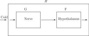
3. You shiver in a cold environment. You step into a cold environment and cold receptors (temperature sensitive nerves with peak response at 30°C) send signals to your hypothalamus; the hypothalamus causes signals to be sent to muscles, increasing their tone; once the tone reaches a threshold, rhythmic muscle contractions begin. See Figure 2.13.
4. Severity of allergenic diseases is increasing. Childhood respiratory infections such as measles, whooping cough, and tuberculosis stimulate a helper T-cell, T#l activity. Increased T#l activity inhibits T#2 (another helper T-cell) activity. Absence of childhood respiratory diseases thus releases T#2 activity. But T H 2 activity increases immunoglobulin E which is a component of allergenic diseases of asthma, hay fever, and eczema. Thus reducing childhood respiratory infections may partially account for the observed recent increase in severity of allergenic diseases 4 .
Definition 2.7.1 Composition of Functions. If F and G are two functions and the domain of F contains part of the range of G, then the composition of F with G is the function, H, defined by
H{x) = F(G(x)) for all x for which G(x) is in the domain of F
The composition, H, is denoted by F o G.
The notation F o G for the composition of F with G means that
(F o G) (x) = F{G{x))
The parentheses enclosing F o G insures that F o G is thought of as a single object (function). The parentheses usually are omitted and one sees
FoG{x) =F(G{x))
3 see the Web page, http://www.heartdisease.org/Traits.html 4 Shirakawa, T. et al, Science 275 1997, 77-79.
CHAPTER 2. DESCRIPTIONS OF BIOLOGICAL PATTERNS
86
Without the parentheses, the novice reader may not know which of the following two ways to group
(FoG)(x) or Fo(G(x))
The experienced reader knows the right hand way does not have meaning, so the left hand way must be correct.
In the “shivering example” above, the nerve cells that perceive the low temperature are the function G and the hypothalamus that sends signals to the muscle is the function F. The net result is that the cold signal increases the muscle tone. This relation may be diagrammed as in Figure 2.13. The arrows show the direction of information flow.
Shivering
Figure 2.13: Diagram of the composition of F – increase of muscle tone by the hypothalamus – with G – stimulation from nerve cells by cold.
Formulas for function composition.
It is helpful to recognize that a complex equation defining a function is a composition of simple parts. For example
H(x) = Vl-x 2
is the composition of
F( z ) = J~z and G{x) = 1 – x 2 F(G(x)) = Vl – x 2
The domain of G is all numbers but the domain of F is only z > 0 and the domain of F o G is only -1 < x < 1.
The order of function composition is very important. For
F(z) = \fz and G[x) = 1 — x 2 , the composition, G o F is quite different from F o G.
and its graph is a semicircle.
G o F{z) = G(F(z)) = 1 – (F(z)) 2 = 1 – (v^) 2 = 1 – z,
and its graph is part of a line (defined for z > 0).
Occasionally it is useful to recognize that a function is the composition of three functions, as in
K{x) = log(sin(:r 2 ))
K is the composition, F o G o H where
F(u) = log(-u) G(v) = sin(t>) H(x) = x 2
The composition of F and F _1 . The composition of a function with its inverse is special. The case of F(x) = x 2 , x > 0 with F^ 1 (x) = ^fx is illustrative.
(F o F~ 1 )(x) = F(F~ 1 (x)) = F(y/x) = [yx^j 2 = x for x > 0
Also
(F” 1 o F)(x) = F-\F(x)) = F~ 1 (x 2 ) = Vx^ = x for x > 0
The identity function I is defined by
I(x) = x for a; in a domain D (2.9) where the domain D is adaptable to the problem at hand.
For F(x) = x 2 and F~ 1 (x) = yfx, F o F~ 1 (x) = F” 1 o F(x) = x = I(x), where D should be x > 0. In the next paragraph we show that
F o F^ 1 = I and F’ 1 o F — I (2.10)
for all invertible functions F.
The ordered pair (a, 6) belongs to F~ l if and only if {b, a) belongs to F. Then
(FoF1 )(a)=F(F-\a))=F(b) = a and (F” 1 o F){b) = F~ 1 (F(b)) = F^ 1 (a) = b
Always, F o F” 1 = I and with an appropriate domain D for /. Also F~ l o F — I with possibly a different domain D for /.
Example 2.7.1 Two properties of the logarithm and exponential functions are
(a) \og b b x = X and (b) u = b l ° s » u
The logarithm function, L(x) = \og b (x) is the inverse of the exponential function, E(x) = b x , and the properties simply state that
LoE = 1 andFoL = J I
CHAPTER 2. DESCRIPTIONS OF BIOLOGICAL PATTERNS
88
The identity function composes in a special way with other functions.
(F o I)(x) = F(I(x)) = F(x) and (I o F)(x) = I(F(x)) = F(x)
Thus
Fol = F and IoF = F Because 1 in the numbers has the property that
ixl = i and 1×1 = 3;
the number 1 is the identity for multiplication. Sometimes F o G is thought of as multiplication also and / has the property analogous to 1 of the real numbers. Finally the analogy of
xx’ 1 = x- = 1 with F o F” 1 = I
x
suggests a rationale for the symbol F^ 1 for the inverse of F.
With respect to function composition F o G as multiplication, recall the example of F(x) = \fx and G(x) = 1 — x 2 in which F o G and G o F were two different functions. Composition of functions is not commutative, a property of real number multiplication that does not extend to function composition.
Exercises for Section 2.7 Composition of functions
Exercise 2.7.1 Four examples of composition of two biological processes (of two functions) were described at the beginning of this section on page 85. Write another example of the composition of two biological processes.
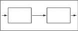
Exercise 2.7.2 Put labels on the diagrams in Figure Ex. 2.7.2 to illustrate the dependence of coyote numbers on rabbit Myxomatosis cuniculi and the dependence of the frequency of heart attacks on diet of a population.
Figure for Exercise 2.7.2 Diagrams for Exercise 2.7.2
Exercise 2.7.3 a. In Explore 1.5.1 of Section 1.5 on page 25 you measured the area of the mold colony as a function of day. Using the same pictures in Figure 1.14, measure the diameters of the mold colony as a function of day and record them in Exercise Table 2.7.3. Remember that grid lines are separated by 2mm. Then use the formula, A = nr 2 , for the area of a circle to compute the third column showing area as a function of day.
b. Determine the dependence of the colony diameter on time.
c. Use the composition of the relation between the area and diameter of a circle (A = 7rr 2 ) with the dependence of the colony diameter on time to describe the dependence of colony area on time.
CHAPTER 2. DESCRIPTIONS OF BIOLOGICAL PATTERNS
Table for Exercise 2.7.3 Table for Exercise 2.7.3
89
Exercise 2.7.4 S. F. Elena, V. S. Cooper, and R. E. Lenski have grown an V. natriegens population for 3000 generations in a constant, nutrient limited environment. They have measured cell size and fitness of cell size and report (Science 272, 1996, 1802-1804) data shown in the graphs below. The thrust of their report is the observed abrupt changes in fitness, supporting the hypothesis of “punctuated evolution.”
a. Make a table showing cell size as a function of time for generations 0, 100, 200, 300, 400 and 500.
b. Make a table showing fitness as a function of time for generations 0, 100, 200, 300, 400 and 500.
c. Are the data consistent with the hypothesis of ‘punctuated equilibrium’ ?
1.4-
0.70 0.65 0.60 $ 0.55 3 0.50 O 0.45 0.40 0.35 0.30
1.3
£ 1.2-
1.1
1.0-
••••
• %
0 500 1000 1500 2000 2500 3000
Time (generations)
0.30 0.35 0.40 0.45 0.50 0.55 0.60 Cell size (fl)
Exercise 2.7.5 Find functions, F(z) and G(x) so that the following functions, H, may be written as F(G(x)).
a. H(x) = (l + x 2 f b. H(x) = 10^ c. H(x) = log (2a; 2 + 1) d. H(x) = Vx^+l e. H{x) = f. H(x) = \og 2 (2 x )
Exercise 2.7.6 Find functions, F(u) and G(v) and H(x) so that the following functions, K, may be written as F(G(H(x))).
a. K{x) = Jl-y/x b. K{x) = (1 + 2 x f c. K{x) = log(2a; 2 + l) d. K(x) = Vx ir Tl e. K(x) = (1 – 2 x f f. K{x) = log 2 (1 + 2 X )
CHAPTER 2. DESCRIPTIONS OF BIOLOGICAL PATTERNS
90
Exercise 2.7.7 Compute the compositions, f(g(x)), of the following pairs of functions. In each case specify the domain and range of the composite function, and sketch the graph. Your calculator may assist you. For example, the graph of part A can be drawn on the TI-86 calculator with GRAPH , y(x) = , yl = x~2 , y2 = l/(l+yl) You may wish to suppress the display of yl with SELCT in the y(x)= menu.
Exercise 2.7.8 For each part, find two pairs, F and G, so that F o G is H
1
a H(x)
d H(x)
(x^y
b H(x)
H(x)
l-y/x
2 (2 )
H(x) = (1+x 2 ) 3
f H(x)
(2 X )2
Exercise 2.7.9 Air is flowing into a spherical balloon at the rate of 10 cm 3 /s. What volume of air is in the balloon t seconds after there was no air in the balloon? The volume of a sphere of radius r is V = iirr 3 . What will be the radius of the balloon t seconds after there is no air in the balloon?
Exercise 2.7.10 Why are all the points of the graph of y = log 10 (sin(x)) on or below the X-axis? Why are there no points of the graph with x-coordinates between n and 2n7
Exercise 2.7.11 Technology Draw the graph of the composition of F(x) = 10 x with G(x) = log 10 x. Now draw the graph of the composition of G with F. Explain the difference between the two graphs.
Exercise 2.7.12 Let P(x) = 2x 3 — 7x 2 + 5 and Q(x) = x 2 — x. Use algebra to compute Q(P(x)). You may conclude (correctly) from this exercise that the composition of two polynomials is always a polynomial.
Exercise 2.7.13 Shown in Figure 2.7.13 is the graph of a function, G. Sketch the graphs of
a. G a (x) = -3 + G(x)
c. G c (x) = 2G(x)
e. G e (x) = 5-2G(x)
g. G g (x) = 3 + G(2(x- 3)
b. d. f. h.
G b (x) G d {x) Gf(x) G h (x)
G((x-3)) G(2 x) G{2 (x-3)) 4 + G(x + 4)
Figure for Exercise 2.7.13 Graph of G for Exercise 2.7.13.
CHAPTER 2. DESCRIPTIONS OF BIOLOGICAL PATTERNS
91

-4 1 ‘ 1 1 ‘ 1 1 1
-4 -2 0 2 4 6 8
2.8 Periodic functions and oscillations.
There are many periodic phenomena in the biological sciences. Examples include wingbeat of insects and of birds, nerve action potentials, heart beat, breathing, rapid eye movement sleep, circadian rhythms (sleep-wake cycles), women’s menstrual cycle, bird migrations, measles incidence, locust emergence. All of these examples are periodic repetition with time, the variable usually associated with periodicity. The examples are listed in order of increasing period of repetition in Table 2.8.
Table 2.8: Characteristic periods of time-periodic biological processes.
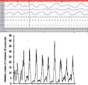
A measurement usually quantifies the state of a process periodic with time and defines a function characteristic of the process. Some examples are shown in Figure 2.14. The measurement may be of physical character as in electrocardiograms, categorical as in stages of sleep, or biological as in measurement of hormonal level.
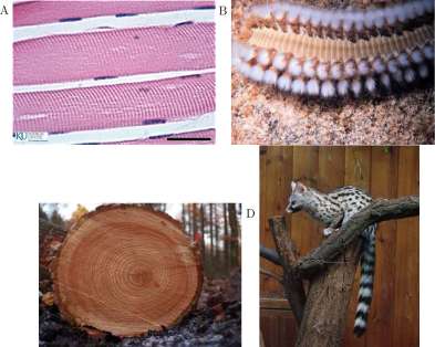
There are also periodic variations with space that result in the color patterns on animals -stripes on zebras and tigers, spots on leopards – , regular spacing of nesting sites, muscle striations, segments in a segmented worm, branching in nerve fibers, and the five fold symmetry of echinoderms. Some spatially periodic structures are driven by time-periodic phenomena – branches in a tree, annular tree rings, chambers in a nautilus, ornamentation on a snail shell. The pictures in Figure 2.8 illustrate some periodic functions that vary with linear space. The brittle star shown in Figure 2.16 varies periodically with angular change in space.
In all instances there is an independent variable, generally time or space, and a dependent variable that is said to be periodic.
CHAPTER 2. DESCRIPTIONS OF BIOLOGICAL PATTERNS
92
A
Wall: mi
■ 1
Mg! rCar’«riia’1lK«!rv-
mi «u
Mb IM&
* in ml
B
. JjyL^J^^—■Jf A -v j\—^—*|S—p—’p/~ j r n ‘—* A-^|
I*

c
D
1948 1960 1952 1954 1956 1958 1960 1962 1964 1966 1968 Year
Figure 2.14: Figures demonstrating periodic repetition with time. (A) Electorcardio-gram. http://en.wikipedia.org/wiki/Electrocardiography uploaded by MoodyGroove. (B) This is a screenshot of a polysomnographic record (30 seconds) representing Rapid Eye Movement Sleep. EEG highlighted by red box. Eye movements highlighted by red line. http://en.wikipedia.Org/wiki/File:REM.png uploaded by Mr. Sandman. (C) Tidal movement 12 hr) (http://en.wikipedia.org/wiki/Tide), uploaded from NOAA, http://co-ops.nos.noaa.gov/images/restfig6.gif. (D) Recurrent epidemics of measles (~2 yr), Anderson and May, Vaccination and herd immunity to infectious diseases, Nature 318 1985, pp 323-9, Figure la.
Definition 2.8.1 Periodic Function. A function, F, is said to be periodic if there is a positive number, p, such that for every number x in the domain of F, x + p is also in the domain of F and
F(x + p) = F(x). (2.11)
and for each number q where 0 < q < p there is some x in the domain of F for which
F(x + q) ^ F(x)
The period of F is p.
The amplitude of a periodic function F is one-half the difference between the largest and least values of F(t), when these values exist.
The condition that ‘for every number x in the domain of F, x + p is also in the domain of F’ implies that the domain of F is infinite in extent — it has no upper bound. Obviously, all of the
CHAPTER 2. DESCRIPTIONS OF BIOLOGICAL PATTERNS
93
C
Figure 2.15: Figures demonstrating periodic repetition with
space. A. Muscle striations, Kansas University Medical School,
http://www.kumc.edu/instruction/medi...r/muscle02.htm. B. Bristle worm, http://www.photolib.noaa.gov/htmls/reefl016.htmlmage ID: reefl016, Dr. Anthony R. Pic-ciolo. C. Annular rings, uploaded by Arnoldius to commons.wikimedia.org/wiki D. A common genet (Genetta genetta), http://en.wikipedia.org/wiki/File:Ge..._(Wroclaw_zoo). JPG Uploaded by Guerin Nicolas. Note a periodic distribution of spots on the body and stripes on the tail.
examples that we experience are finite in extent and do not satisfy Definition 2.8.1. We will use ‘periodic’ even though we do not meet this requirement.
The condition ‘when these numbers exist’ in the definition of amplitude is technical and illustrated in Figure 2.17 by the graph of
F(t) = t-[t]
where [t] denotes the integer part of t. ([tt] = 3, [y/30] = 5). There is no largest value of F(t).
F{n) = n — [n] = 0 for integer n
If t is such that F(t) is the largest value of F then t is not an integer and is between an integer n and Ti+l. The midpoint s of [t,n + 1] has the property that F(t) < F(s), so that F(t) is not the largest value of F.
CHAPTER 2. DESCRIPTIONS OF BIOLOGICAL PATTERNS
94
Figure 2.16: A. Periodic distribution of Gannet nests in New Zealand. B. A star fish demonstrating angular periodicity, NOAA’s Coral Kingdom Collection, Dr. James P. McVey, http://www.photolib.noaa.gov/htmls/reef0296.htm.
F(t)=t-[t]
Figure 2.17: The graph of F(t) = t — [t] has no highest point.
The function, F(t) = t — [t] is pretty clearly periodic of period 1, and we might say that its amplitude is 0.5 even though it does not satisfy the definition for amplitude. Another periodic function that has no amplitude is the tangent function from trigonometry.
Periodic Extension Periodic functions in nature do not strictly satisfy Definition 2.8.1, but can be approximated with strictly periodic functions over a finite interval of their domain. Periodic functions in nature also seldom have simple equation descriptions. However, one can sometimes describe the function over one period and then assert that the function is periodic – thus describing the entire function.
Example 2.8.1 Electrocardiograms have a very characteristic periodic signal as shown in Figure 2.14.
A picture of a typical signal from ‘channel I’ is shown in Figure 2.18; the regions of the signal, P-R, QRS, etc. correspond to electrical events in the heart that cause contractions of specific muscles. Is there an equation for such a signal? Yes, a very messy one!
The graph of the following equation is shown in Figure 2.18(b). It is similar to the typical
CHAPTER 2. DESCRIPTIONS OF BIOLOGICAL PATTERNS
95
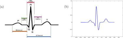
Figure 2.18: (a) Typical signal from an electrocardiogram, created by Agateller (Anthony Atkielski) http://en.wikipedia.org/wiki/Electrocardiography, . (b) Graph of Equation 2.12
electrocardiogram in Figure 2.18(a).
H(t) = 25000 + 0.05) t (t – 0^.07) + Q 15 2 -i 60 o( i+ o.i75)^ + Q 25 2 -90o (t -o.2)^
(l + (20t) 10 ) 2 1 2 ) (212)
-0.4 < t < 0.4
Explore 2.8.1 Technology Draw the graph of the heart beat Equation 2.12. You will find it useful to break the function into parts. It is useful to define
= 2500Q (. + 0.05), (,- 0.07) (l + (20x) 10 )
y2 = (yl)/2\ Z )
and y3 and yA for the other two terms, then combine y2, y3 and yA into yb and select only y5 to graph. ■
The heart beat function H in Equation 2.12 is not a periodic function and is defined only for —0.4 <t< 0.4. Outside that interval, the expression defining H(t) is essentially zero. However, we can simultaneously extend the definition of H and make it periodic by
H{t) = Hit – 0.8) for all t
What is the impact of this? i?(0.6), say is now defined, to be H(— 0.2). Immediately, H has meaning for 0.4 <t< 1.2, and the graph is shown in Figure 2.19(a). Now because H(t) has meaning on 0.4 < t < 1.2, H also has meaning on 0.4 < t < 2.0 and the graph is shown in Figure 2.19(b). The extension continues indefinitely, h ■
Definition 2.8.2 Periodic extension of a function. If f is a function defined on an interval [a,b) and p = b — a, the periodic extension of F of f is defined by
F(t) = f(t) for a < t < b, F(t + p) = F(t) for -oo <t < oo { }
CHAPTER 2. DESCRIPTIONS OF BIOLOGICAL PATTERNS
96
-0.4 -0.2 0 0.2 0.4 0.6 0.B 1 1.2 1.4 -0.5 O 0.5 1 1.5 2
Figure 2.19: (a) Periodic extension of the heart beat function H of Equation 2.12 by one period, (a) Periodic extension of the heart beat function H to two periods.
Equation 2.13 is used recursively. For t in \ab), t + p is in [b,b + p) and Equation 2.13 defines F on [6, b + p). Then, for t in [b, b + p), t + p is in [b + p, b + 2p) and Equation 2.13 defines F on [b + p, b + 2p). Continue this for all values of t > b. If t is in [a — p, a) then t + p is in [a, b) and F(t) = F(t + p). Continuing in this way, F is defined for all t less than a.
Exercises for Section 2.8, Periodic functions and oscillations.
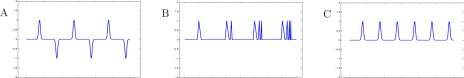
Exercise 2.8.1 Which of the three graphs in Figure Ex. 2.8.1 are periodic. For any that is periodic, find the period and the amplitude.
Figure for Exercise 2.8.1 Three graphs for Exercise 2.8.1 .
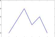
Exercise 2.8.2 Shown in Figure Ex. 2.8.2 is the graph of a function, / defined on the interval [1,6]. Let F be the periodic extension of /.
a. What is the period of Fl
b. Draw a graph of F over three periods.
c. Evaluate F(l), F(3), F(8), F(23), F(31) and F(1004).
d. Find the amplitude of F.
Figure for Exercise 2.8.2 Graph of a function / for Exercise 2.8.2
CHAPTER 2. DESCRIPTIONS OF BIOLOGICAL PATTERNS
0 1 2 3 4 5 6 7
Exercise 2.8.3 Suppose your are traveling an interstate highway and that every 10 miles there an emergency telephone. Let D be the function defined by
D(x) is the distance to the nearest emergency telephone
where x is the mileage position on the highway.
a. Draw a graph of D.
b. Find the period and amplitude of D.
Exercise 2.8.4 Your 26 inch diameter bicycle wheel has a patch on it. Let P be the function defined by
P(x) is the distance from patch to the ground where x is the distance you have traveled on a bicycle trail.
a. Draw a graph of P (approximate is acceptable).
b. Find the period and amplitude of P.
Exercise 2.8.5 Let F be the function defined for all numbers, x, by
F(x) = the distance from x to the even integer nearest x.
a. Draw a graph of F.
b. Find the period and amplitude of F.
Exercise 2.8.6 Let / be the function defined by
f(x) = l-x 2 – 1 < x < 1 Let F be the extension of / with period 2.
a. Draw a graph of /.
b. Draw a graph of F.
c. Evaluate F(l), F(2), F(3), F(12), F(31) and F(1002).
d. Find the amplitude of F.
CHAPTER 2. DESCRIPTIONS OF BIOLOGICAL PATTERNS
98
2.8.1 Trigonometric Functions.
The trigonometric functions are perhaps the most familiar periodic functions and often are used to describe periodic behavior. However, not many of the periodic functions in biology are as simple as the trigonometric functions, even over restricted domains.
Amplitude and period and frequency of a Cosine Function. The
function
H{t) = A cos C-^-t + <f?j A>0 P>0 and 0 any angle has amplitude A, period P, and frequency 1/P.
Graphs of rescaled cosine functions shown in Figure 2.20 demonstrate the effects of A and P.
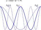
3rc/2 2tc
Figure 2.20: (a) Graphs of the cosine function for amplitudes 0,5 1.5 and 1.5. (b) Graphs of the cosine function for periods 0.5, 1.0 and 2.0.
Example 2.8.2 Problem. Find the period, frequency, and amplitude of
Hit) = 3 sin(5t + vr/3) Solution. Write Hit) = 3sin(5t + 7r/3) as
i/(t) = 3sin (J75 t + ,r/3 )^
Then the amplitude of P is 3, and the period is 27r/5 and the frequency is 5/(27r). ■
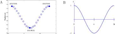
Motion of a Spring-Mass System A mass suspended from a spring, when vertically displaced from equilibrium a small amount will oscillate above and below the equilibrium position. A graph of displacement from equilibrium vs time is shown in in Figure 2.21A for a certain system. Critical points of the graph are
(2.62 s, 72.82 cm), (3.18 s, 46.24 cm), and (3.79 s, 72.80 cm)
CHAPTER 2. DESCRIPTIONS OF BIOLOGICAL PATTERNS
99
Time sec
Figure 2.21: Graphs of A. the motion of a spring-mass system and B. H(t) = cost.
Also shown is the graph of the cosine function, H(t) = cost.
It is clear that the data and the cosine in Figure 2.21 have similar shapes, but examine the axes labels and see that their periods and amplitudes are different and the graphs lie in different regions of the plane. We wish to obtain a variation of the cosine function that will match the data.
The period of the harmonic motion is 3.79 – 2.62 = 1.17 seconds, the time of the second peak minus the time of the first peak. The amplitude of the harmonic motion is
0.5(72.82 — 46.24) = 13.29 cm, one-half the difference of the heights of the highest and lowest points. Now we expect a function of the form
H 0 (t) = 13.3cos(^t)
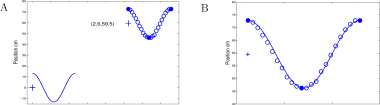
to have the shape of the data, but we need to translate vertically and horizontally to match the data. The graphs of Hq and the data are shown in Figure 2.22A, and the shapes are similar. We need to match the origin (0,0) with the corresponding point (2.62, 59.5) of the data. We write
H(t) = 59.5 + 13.3 cos (j^(t ~ 2.62)) The graphs of H and the data are shown in Figure 2.22B and there is a good match.
Time sec Time sec
Figure 2.22: On the left is the graph of Ho(t) = 13.3 cos \ Yrft\ and the harmonic oscillation data. The two are similar in form. The graph to the right shows the translation, H, of H 0 , Hit) = 59.5 + 13.3 cos [jfvit ~ 2.62)) and its approximation to the harmonic oscillation data.
CHAPTER 2. DESCRIPTIONS OF BIOLOGICAL PATTERNS
100
Polynomial approximations to the sine and cosine functions. Shown in Figure 2.23 are the graphs of F(x) = sinx and the graph of (dashed curve)
Pr(x)
x
X
120
on [0,7r/2].
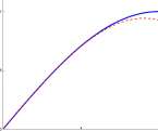
Figure 2.23: The graphs of F(x) = sinx (solid) and P 3 (x) = x — ^ (dashed) on [0, ir/2]
The graph of P 3 is hardly distinguishable from the graph of F on the interval [0,7r/4], although they do separate near x = tt/2. F(x) = sinx is difficult to evaluate (without a calculator) except for special values such as F(0) = sinO = 0, F(ir/3) = sin7r/3 = 0.5 and F(tt/2) = sin7r/2 = 1.0. However, P 3 (x) can be calculated using only multiplication, division and subtraction. The maximum difference between P 3 and F on [0,tt/4] occurs at tt/4 and F(tt/4) = ^2/2 = 0.70711 and P 3 (7r/4) = 0.70465. The relative error in using P 3 (7r/4) as an approximation to F(n/4) is
|P 3 (7r/4) -F(ir/4)\ 10.70465 — 0.707111
Relative Error = 1 3V ‘J, , t C 1 n = l – — l – = 0.0036
F(?r/4) 0.70711
thus less than 0.5% error is made in using the rather simple P 3 (x) = x — (x 3 )/120 in place of F(x) = sinx on [0,7r/4].
Exercises for Section 2.8.1, Trigonometric functions.
Exercise 2.8.7 Find the periods of the following functions.
a. P(t) = sin(ft) d. P(t) = sin(t) + cos(t)
b. P(t) = sm(t) e. P(t) = sin(^t) + sin(^t)
c. P(t) = 5-2sin(t) f. P(t) = tan2t
Exercise 2.8.8 Sketch the graphs and label the axes for
(a) y = 0.2cos ^— 1\ and (b) y = 5cos ^-t + vr/6
Exercise 2.8.9 Describe how the harmonic data of Figure 2.22A would be translated so that the graph of the new data would match that of H 0 .
Exercise 2.8.10 Use the identity, cost = sin(t + |), to write a sine function that approximates the harmonic oscillation data.
CHAPTER 2. DESCRIPTIONS OF BIOLOGICAL PATTERNS
101
Exercise 2.8.11 Fit a cosine function to the spring-mass oscillation shown in Exercise Figure 2.8.11.
Figure for Exercise 2.8.11 Graph of a spring-mass oscillation for Exercise 2.8.11.
(2.4,68.6)
70 –
0 o« 0
(1.8,50.9)
(3.0,51.0)
2 2.2 2.4 2.6 2.B 3 3.2
Time s
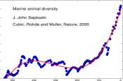
Exercise 2.8.12 A graph of total marine animal diversity over the period from 543 million years ago until today is shown in Exercise Figure 2.8.12A. The data appeared in a paper by Robert A. Rohde and Richard A. Muller 5 , and are based on work by J. John Sepkoski 6 . Also shown is a cubic polynomial fit to the data by Robert Rohde and Richard Muller who were interested in the the difference between the data and the cubic shown in Exercise Figure 2.8.12B. They found that a sine function of period 62 million years fit the residuals rather well. Find an equation of such a sine function.
Figure for Exercise 2.8.12 A. Marine animal diversity and a cubic polynomial fit to the data. B. The residuals of the cubic fit. Figures adapted from Robert A. Rohde and Richard A. Muller, Cycles in fossil diversity, Nature 434, 208-210, Copyright 2005, http://www.nature.com
A
Marine animal diversity J. John Sepkoski
Cubic: Rohde and Muller, Nature, 2005
B
0
\ .’..V •/* .;V*V* V
Rhode and Muller, Nature, 2005
Million Years Ago
Million Years Ago
Exercise 2.8.13 Technology Draw the graphs of F(x) = sin a; and
F(x) = sin a; and Pr(x) = x 1
K J 5V ‘ 6 120
on the range 0 < x < tt. Compute the relative error in P 5 (7r/4) as an approximation to F(n/4) and in P${ii/2) as an approximation to F{ti/2).
Exercise 2.8.14 Technology Polynomial approximations to the cosine function. 5 Robert A. Rohde and Richard A. Muller, Cycles in fossil diversity, Nature 434, 208-210.
6 J. John Sepkoski, A compendium of Fossil Marine Animal Genera, Eds David Jablonski and Michael Foote, Bulletins of AMerican Paleontology, 363, 2002.
CHAPTER 2. DESCRIPTIONS OF BIOLOGICAL PATTERNS
102
a. Draw the graphs of F(x) = cos re and
x 2
F(x) = cosx and P2{x) = 1 ——
on the range 0 < x < it.
b. Compute the relative error in P 2 (tt/4) as an approximation to F(ir/4) and in P 2 (it/2) as an approximation to F(ir/2).
c. Use a graphing calculator to draw the graphs of F(x) = cosx and
2 4
on the range 0 < x < it.
d. Compute the relative error in P 4 (7r/4) as an approximation to F{ix/A) and the absolute error in P^n /2) as an approximation to F(tt/2).
Chapter 3
The Derivative
Calculus is the study of change and rates of change. It has two primitive concepts, the derivative and the integral. Given a function relating a dependent variable to an independent variable, the derivative is the rate of change of the dependent variable as the independent variable changes. We determine the derivative of a function when we answer questions such as
1. Given population size as a function of time, at what rate is the population growing?
2. Given the position of a particle as a function of time, what is its velocity?
CHAPTER 3. THE DERIVATIVE
104
3. At what rate does air density decrease with increasing altitude?
4. At what rate does the pressure of one mole of O2 at 300°K change as the volume changes if the temperature is constant?
On the other hand, given the rate of change of a dependent variable as an independent variable changes, the integral is the function that relates the dependent variable to the independent variable.
1. Given the growth rate of a population at all times in a time interval, how much did the population size change during that time interval?
2. Given the rate of renal clearance of penicillin during the four hours following an initial injection, what will be the plasma penicillin level at the end of that four hour interval?
3. Given that a car left Chicago at 1:00 pm traveling west on 180 and given the velocity of the car between 1 and 5 pm, where was the car at 5 pm?
The derivative is the subject of this chapter; the integral is addressed in Chapter 9. The derivative and integral are independently defined. Chapter 9 can be studied before this one and without reference to this one. The two concepts are closely related, however, and the relation between them is The Fundamental Theorem of Calculus, developed in Chapter 10.
Explore 3.0.2 You use both the derivative and integral concepts of calculus when you cross a busy street. You observe the nearest oncoming car and subconsciously estimate its distance from you and its speed (use of the derivative), and you decide whether you have time to cross the street before the car arrives at your position (a simple use of the integral). Might there be a car different from the nearest car that will affect your estimate of the time available to cross the street? You may even observe that the car is slowing down and you may estimate whether it will stop before it gets to your crossing point (involves the integral). It gets really difficult when you are traveling on a two-lane road and want to pass a car in front of you and there is an oncoming vehicle. Teenage drivers learn calculus.
Give an example in which estimates of distances and speeds and times are important for successful performance in a sport. ■
3.1 Tangent to the graph of a function
CHAPTER 3. THE DERIVATIVE
105
Elementary and very important.
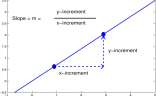
Consider a line with equation, y = m x + b.
The slope, m, of the line is computed as the increment in y divided by the increment in x between two points of the line, and may be called the rate of change of y with respect to x.
• If y measures bacterial population size at time x measured in hours, the slope m is the bacterial increase per hour, or bacterial growth rate, with dimensions, pop/hour.
• If y measures the height of a young girl in inches at year x, then m is the growth rate of the girl in inches per year.
• If y measures a morphogen concentration a distance x from its source in a developing embryo, m is the rate of concentration decrease, called a morphogenetic gradient, that causes differentiation of specific cell types in a distinct spatial order.
The simple rate of change of linear functions is crucial to understanding the rate of change of nonlinear functions.
Example 3.1.1 At what rate was the Vibrio natriegens population of Section 1.1 growing at time T = 40 minutes?
We have data for population density (measured in absorbance units) at times T = 0, T = 16, T = 32, T = 48, T = 64, and T = 80, minutes.
Time 0 16 32 48 64 80 Absorbance 0.022 0.036 0.060 0.101 0.169 0.266
The average growth rate between times T = 32 and T = 48 is
0.101 — 0.060 Absorbance units
= 0.0026 ,
48 – 32 minute
and is a pretty good estimate of the growth rate at time T = 40, particularly because 40 is midway between 32 and 48.
In Section 1.1 we let t index time in 16 minutes intervals, and we used the mathematical model that population increase during time t to t + 1 is proportional to the population at time t. With B t being population at time index t, we wrote
B t+1 -B t = rxB t for t = 0,1, 2, 3,4, 5,
CHAPTER 3. THE DERIVATIVE
106
We concluded that
B t = 0.022 for
t = 0,1,2,3,4,5.
In terms of T in minutes and 5(T) in absorbance units, (Equation 1.5)
. 5 xT/16
/5\ ‘
5(T) = 0.022 I-J = 0.022 ■ 1.032 5
(3.1)
(3.2)
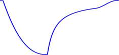
Shown in Figure 3.1 A are the data, the discrete computations of Equation 3.1 and the graph of Equation 3.2. A magnification of the graph near T = 40 minutes is shown Figure 3. IB together with a tangent drawn at (40, 5(40)).
A
B
20 30 40 50
Time — minutes
Time — minutes
Figure 3.1: A. Graph of the V. natriegens data (+), the discrete approximation of Equation 3.1 (filled circles) and the graph of Equation 3.2. A magnification near T = 40 minutes is shown in B together with a tangent to the graph of 5(T) (Equation 3.2) at (40,5(40)).
We define the (instantaneous) growth rate of a population described by B(T) at time T = 40 to be the slope of the tangent to the graph of B at time T = 40. The units on the slope of the tangent are
change in y Absorbance units
change in x Time in seconds
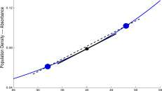
and are appropriate for population growth rate. Shown in Figure 3.2 are the tangent and a secant line between ( 32,5(32)) and (48,5(48)). The slope of the secant is
= °10185 -°06111 = 0.002546 48 – 32 16
This is the average growth rate of 5 and is slightly different from the average growth rate (0.0026) computed from the data because 5 only approximates the data (pretty well, actually) and can be computed with higher accuracy than is possible with the data.
We can compute a closer estimate of the slope of the tangent by computing
5(45j-5(35) = 0.092549 -0.067254 = 45 – 35 10
It would be possible to have absorbance data at 5 minute intervals and compute the average growth rate between 35 and 45 minutes, but there are two difficulties. The main difficulty is that absorbance (on our machine) can only be measured to three decimal digits and the answer could be
CHAPTER 3. THE DERIVATIVE
107
Time — minutes
Figure 3.2: Graph of B(T), the tangent to the graph at (40,5(40)) and the secant through (32,5(32)) and (48,5(48)).
trusted to only 3 decimal digits, the first of which is 0. A second problem is that at each reading, 10 ml of growth serum is extracted, analyzed in the spectrophotemeter, and discarded. In 80 minutes, 160 ml of serum would be discarded, possibly more than was initially present.
Example 3.1.2 At what rate was the world human population increasing in 1980? Shown in Figure 3.3 are data for the twentieth century and a graph of an approximating function, F. A tangent to the graph of F at (1980, F(1980)) is drawn and has a slope of 0.0781 • 10 9 = 78,100, 000 . Now,
rise change in population people
slope is = : « .
run change m years year
The units of slope, then, are people/year. Therefore,
slope = 78,100,000 pe0ple ,
year
The world population was increasing approximately 78,100,000 people per year in 1980. Explore 3.1.1 At approximately what rate was the world human population increasing in 1920?
Definition 3.1.1 Rate of change of a function at a point. If the graph of a function, F, has a tangent at a point (a, F(a)), then the rate of change of F at a is the slope of the tangent to F at the point (a,F(a)).
CHAPTER 3. THE DERIVATIVE
108
D- 3.5
I 3
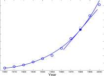
Figure 3.3: Graph of United Nations estimates of world human population for the twentieth century, an approximating curve, and a tangent to the curve. The slope of the tangent is 0.0781 ■ 10 9 = 78,100,000.
A
(3,2)
B
(3,2)
c 3
(3,2)
Figure 3.4: In neither of these graphs will we accept a line as tangent to the graph at the point (2,3)
To be of use, Definition 3.1.1 requires a definition of tangent to a graph which is given below in Definition 3.1.3. In some cases there will be no tangent. In each graph shown in Figure 3.4 there is no tangent at the point (3,2) of the graph. Students usually agree that there is no tangent in graphs A and B, but sometimes argue about case C.
Explore 3.1.2 Do you agree that there is no line tangent to any of the graphs in Figure 3.4 at the point (3,2)? ■
Examples of tangents to graphs are shown in Figure 3.5; all the graphs have tangents at the point (2,4). In Figure 3.5C, however, the line shown is not the tangent line. The graphs in B and C are the same and the tangent at (2, 4) is the line drawn in B.
A line tangent to the graph of F at a point (a, F(a)) contains (a, F(a)) so in order to find the tangent we only need to find the slope of the tangent, which we denote by m a . To find m a we consider points b in the domain of F that are different from a and compute the slopes,
F(b) – F(a)
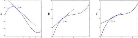
Figure 3.5: All of these graphs have a tangent to the graph at the point (2,4). However, the line drawn in C is not the tangent.
of the lines that contain (a,F(a)) and (b,F(b)). The line containing (a,F(a)) and (b,F(b)) is called
a secant of the graph of F. The slope, _ > °f the secant is a ‘good’ approximation to the slope of the tangent when b is ‘close to’ a. A graph, a tangent to the graph, and a secant to the graph are shown in Figure 3.6. If we could animate that figure, we would slide the point (b, F(b)) along the curve towards (a,F(a)) and show the secant moving toward the tangent.
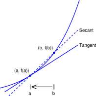
Figure 3.6: A graph, a tangent to the graph, and a secant to the graph.
A substitute for this animation is shown in Figure 3.7. Three points are shown, Bi, B2, and .63 with B\ = (bi,F(bi)), B 2 = (62,^(62))) and B 3 = (6 3 ,F(6 3 )). The numbers b\, b 2 , and 63 are progressively closer to a, and the slopes of the dashed lines from B 1} B 2 , and B 3 to (a,F(a)) are progressively closer to the slope of the tangent to the graph of F at (a, F(a)). Next look at the magnification of F in Figure 3.7B. The progression toward a continues with 63, 64, and 65, and the slopes from B 3 , B±, and B 5 to (a, F(a)) move even closer to the slope of the tangent.
Explore 3.1.3 It is important in Figure 3.7 that as the x-coordinates b\, b 2 , • • • approach a the points B\ = (61, F(bi) ), B 2 = ( b 2 , F(b 2 ) ), • • • on the curve approach (a, /(a)). Would this be true in Figure 3.4B? ■
CHAPTER 3. THE DERIVATIVE
110

Figure 3.7: A. A graph and tangent to the graph at (a,F(a)). Slopes of the secant lines from Bi, B 2 , and B 3 to (a,F(a)) progressively move toward the slope of the tangent. B. A magnification of A with the progression continued.
Definition 3.1.2 Suppose a and b are two numbers and a < b. The open interval, (a, b) consists of all of the numbers between a and b (not including either a or b). The closed interval, [a, b] consists of a, all of the numbers between a and b, and b.
The notation for open interval is ambiguous. (3,5) might represent all the numbers between 3 and 5 or might represent the point in the plane whose coordinate pair is (3,5). The context of it use should clarify its meaning.
Definition 3.1.3 Tangent to a graph. Suppose the domain of a function F contains an open interval that contains a number a. Suppose further that there is a number m a such that that for points b in the interval different from
as 6 approaches a ERzIM approaches m „.
b — a
Then m a is the slope of the tangent to F at (a, F(a)). The graph of y = F(a) + m a (x — a) is the tangent to the graph of F at (a, F(a)).
We are making progress. We now have a definition of tangent to a graph and therefore have riven meaning to rate of change of a function. However, we must make sense of the phrase
CHAPTER 3. THE DERIVATIVE
111
This phrase is a bridge between geometry and analytical computation and is formally defined in Definition 3.2.1. We first use it on an intuitive basis. Some students prefer an alternate, similarly intuitive statement:
., , • , F ( b ) – F ( a ) ■ i
if o is close to a is close to m a .
b — a
Both phrases are helpful.
Consider the parabola, shown in Figure 3.8,
F(t) = t 2 for all t and a point (a, a 2 ) of F.

Secant
Tangent
_i i ‘ ‘ ‘ ‘
-10 12 3
Figure 3.8: The parabola, F(t) = t 2 , a tangent to the parabola at (a,a 2 ), and a secant through (a, a 2 ) and {b,b 2 ).
The slope of the secant is
F(b) – F(a) b 2 -a 2 (b – a) (b + a)
b + a.
b — a b — a b — a
Although ‘approaches’ has not been carefully defined, it should not surprise you if we conclude that
F(b)-F(a) b 2 -a 2 ,
as o approaches a = = b + a approaches a + a = 2a.
b — a b — a
Alternatively, we might conclude that
• , F(b)-F(a) b 2 -a 2 ,
if 6 is close to a = — = b + a is close to a + a = 2a.
b — a b — a
We make either conclusion, and along with it conclude that the slope of the tangent to the parabola y = x 2 at the point (a, a 2 ) is 2a. Furthermore, the rate of change of F(t) = t 2 at a is 2a. This is the first of many examples.
CHAPTER 3. THE DERIVATIVE
112
Explore 3.1.4 Do this. Use your intuition to answer the following questions. You will not answer g. or h. easily, if at all, but think about it.
a. As 6 approaches 4,
b. As 6 approaches 2,
c. If b is close to 5,
d. As b approaches 0,
e. If b is close to 0,
f. As b approaches 0,
g. As b approaches 0, g*. If b is close to 0,
h. As b approaches 0, h*. If b is close to 0,
what number does 3b approach? what number does b 2 approach? what number is 36 + b 3 close to? what number does y approach? what number is 2 b close to? does y approach a number?
what number does approach? Use radian measure of angles, what number is close to? Use radian measure of angles, what number does 2 -F^ approach?
what number is
close to?
One may look for an answer to c, for example, by choosing a number, 6, close to 5 and computing 3 b + 6 3 . Consider 4.99 which some would consider close to 5. Then 3 • 4.99 + 4.99 3 is 139.22. 4.99999 is even closer to 5 and 3 • 4.99999 + 4.99999 3 is 139.99922. One may guess that 3b + 6 3 is close to 140 if b is close to 5. Of course in this case 3b + b 3 can be evaluated for b = 5 and is 140. The approximations seem superfluous.
Explore 3.1.5 Item g*. is more interesting than item c because ^ is meaningless for 6 = 0.
b
Compute ^ for 6 = 0.1, 6 = 0.01, and 6 = 0.001 (put your calculator in radian mode) and answer the question of g*. ■
Item h is more interesting than g*. Look at the following computations.
6 = 0.1 2(U 0 ~ 1 = 0.717734625
oO.Ol i
6 = 0.01 1 Q Q ~ 1 = 0.69555006
o 0.001 i
6 = 0.001 1 Q Q0 ~ 1 = 0.69338746
oO.OOOOOl i
6 = 0.0001 o ooooor = 0.6931474
It is not clear what the numbers on the right are approaching, and, furthermore, the number of digits reported are decreasing. This will be explained when we compute the derivative of the exponential functions in Chapter 5
Explore 3.1.6 Set your calculator to display the maximum number of digits that it will display. Calculate 2 0 00001 and explain why the number of reported digits is decreasing in the previous computations.
Your calculator probably has a button marked ‘LN’ or ‘Ln’ or ‘In’. Use that button to compute In 2 and compare ln 2 with the previous calculations. ■
CHAPTER 3. THE DERIVATIVE
In the next examples, you will find it useful to recall that for numbers a and 6 and n a positive integer,
b n – a n = (6 – a) ( b n ~ x + b n ~ 2 a + 6 n ~ 3 a 2 + ■■■ + 6 2 a n ” 3 + ba n ~’ 2 + a™” 1 ). (3.3)
2„n—3 i L^rt—2 I „n—\
Problem. Find the rate of change of
F(i) = 2t 4 – 3t at t = 2.
Equivalently, find the slope of tangent to the graph of F at the point (2,26). Solution. For b a number different from 2,
F(6) – F(2) {2b 4 – 36) – (2 • 2 4 – 3 • 2)
6-2
We claim that
As 6 approaches 2,
gg) ~ ^(2) 6-2
6-2
6 4 – 2 4 6 -2 2 T^2″” 3 6^2
2f6 3 + 6 2 -2 + 6-2 2 + 2 3 ) -3
2 (6 3 + 6 2 • 2 + 6 • 2 Z + 2 6 ) – 3 approaches 61.
Therefore, the slope of the tangent to the graph of F at (2,26) is 61, and the rate of change of F{t) = 2t A — 3t at t = 2 is 61. An equation of the tangent to the graph of F at (2,26) is
y-26
t – 2
61, y = 61i-96
Graphs of F and y = 61t — 96 are shown in Figure 3.9.
(2,26)
Figure 3.9: Graphs of F(t) = 2t 4 – 3t and the line y = 61* – 96.
Problem. Find an equation of the line tangent to the graph of
F(t) = -J at the point (2,1/4)
CHAPTER 3. THE DERIVATIVE
114
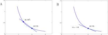
Figure 3.10: A. Graphs of F(t) = 1/t 2 and a secant to the graph through (6, l/b 2 ) and (2,1/4). B. Graphs of F(t) = 1/t 2 and the line y = -I/At + 3/4.
Solution. Graphs of F(t) = 1/t 2 and a secant to the graph through the points (6, l/b 2 ) and (2,1/4) for a number b not equal to 2 are shown in Figure 3.10A. The slope of the secant is
1 1
Fib) – F{2) = tf~2 2 6-2 6-2
2 2 – 6 2 1
6 2 • 2 2 6 – 2 2 + 6
2 2 -6 2
See Equation 3.3
We claim that
t , , F(b)-F(2) 2 + 6 , 1
As 6 approaches 2, — = — ^— ^ approaches — –
An equation of the line containing (2,1/4) with slope -1/4 is
This is an equation of the line tangent to the graph of F(t) = 1/t 2 at the point (2,1/4). Graphs of F and y = — l/4t + 3/4 are shown in Figure 3.1 OB.
Explore 3.1.7 In Explore Figure 3.1.7 is the graph of y = tfx. Does the graph have a tangent at (0,0)? Your vote counts. ■
Explore Figure 3.1.7 Graph of y = yfx.
CHAPTER 3. THE DERIVATIVE
C(t) = t
1/3
(0, 0)
Problem. At what rate is the function F(t) = \/i increasing at t = 8? Solution. For a number 6 not equal to 8,
F{b)-F{8) Vb-^8
6-8
6-8
^6-2 (^6) 3 -2 3
Lightning Bolt! See Figure 3.11
Now we claim that
(^6) 2 + ^6-2 + 2 2
F(b)-F(8) 1 , 1
as 6 approaches 8 , = ^ approaches —.
6-8 (^)2 + ^. 2 + 2 2 PP 12
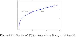
Therefore, the rate of increase of F(t) = ffi at t = 8 is 1/12. A graph of F(t) = \ft and y = t/12 + 4/3is shown in Figure 3.12.
Pattern. In each of the computations that we have shown, we began with an expression for
m – no)
b — a
that was meaningless for 6 = a because of 6 — a in the denominator. We made some algebraic rearrangement that neutralized the factor 6 — a in the denominator and obtained an expression E{b) such that
1. F ^ h \ ~ ^ = E{b) for 6 ^ a, and
2. £?(a) is defined, and
3. As 6 approaches a, E(b) approaches E(a).
CHAPTER 3. THE DERIVATIVE
116
A Lightning Bolt signals a step that is a surprise, mysterious, obscure, or of doubtful validity, or to be proved in later chapters. Think of Zeus atop Mount Olympus issuing thunderous proclamations amid darkness and lightning.

Figure 3.11: Figure of Zeus from http://en.wikipedia.org/wiki/Zeus. Picture is by Sdwelchl031
We then claimed that
F(b) – F(a)
as o approaches a approaches E(a).
b — a
This pattern will serve you well until we consider exponential, logarithmic and trigonometric functions where more than algebraic rearrangement is required to neutralize the factor b — a in the denominator. Item 3 of this list is often given scant attention, but deserves your consideration.
Exercises for Section 3.1, Tangent to the graph of a function.
Exercise 3.1.1 Approximate the growth rate of the V. natriegens population of Table 1.1 at time t = 56 minutes.
Exercise 3.1.2 Approximate the growth rate of B(T) = 0.022 at time a. T = 56 minutes, b. T = 30 minutes, c. T = 0 minutes.
CHAPTER 3. THE DERIVATIVE
117
Exercise 3.1.3 Shown in Exercise Figure 3.1.3 is the ventricular volume of the heart during a normal heart beat of 0.8 seconds. During systole the ventricle contracts and pushes the blood into the aorta. Find approximately the flow rate in ml/sec of blood in the aorta at time t = 0.2 seconds. Find approximately the maximum flow rate of blood in the aorta.
Figure for Exercise 3.1.3 Graph of the ventricular volume during a normal heart beat.
Patterned after the graph in Figure 9.13.
CD
E
\_ 80 CO
Systole
Diastole
0.3 0.4 0.5
Time sec
Exercise 3.1.4 Shown in Exercise Figure 3.1.4 is a graph of air densities in Kg/m 3 as a function of altitude in meters (U.S. Standard Atmospheres 1976, National Oceanic and Atmospheric Administration, NASA, U.S. Air Force, Washington, D.C. October 1976). You will find the rate of change of density with altitude. Because the independent variable is altitude, a distance, the rate of change is commonly called the gradient.
a. At what rate is air density changing with increase of altitude at altitude = 2000 meters? Alternatively, what is the gradient of air density at 2000 meters?
b. What is the gradient of air density at altitude = 5000 meters?
c. What is the gradient of air density at altitude = 8000 meters?
Figure for Exercise 3.1.4 Graph of air density (Kg/m 3 ) vs altitude (m).
53 0 .8
0.7
1000 2000 3000 4000 5000 6000 7000 8000 9000 10000
Altitude meters
CHAPTER 3. THE DERIVATIVE
118
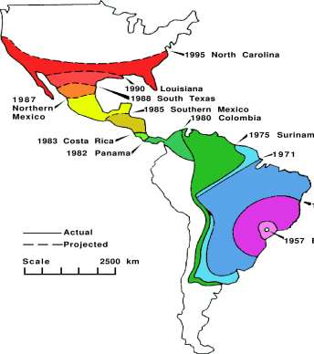
Exercise 3.1.5 An African honey bee Apis mellifera scutellata was introduced into Brazil in 1956 by geneticists who hoped to increase honey production with a cross between the African bee which was native to the tropics and the European species commonly used by bee keepers in South America and in the United States. Twenty six African queens escaped into the wild in 1957 and the subsequent feral population has been very aggressive and has disrupted or eliminated commercial honey production in areas where they have spread.
Shown in Exercise Figure 3.1.5 is a map 1 that shows the regions occupied by the African bee in the years 1957 to 1983, and projections of regions that would be occupied by the bees during 1985-1995.
a. At what rate did the bees advance during 1957 to 1966?
b. At what rate did the bees advance during 1971 to 1975?
c. At what rate did the bees advance during 1980 to 1982?
d. At what rate was it assumed the bees would advance during 1983 – 1987?
Figure for Exercise 3.1.5 The spread of the African bee from Brazil towards North America. The solid curves with dates represent observed spread. The dashed curves and dates are projections
of spread.
1 Orley R. Taylor, African bees: potential impact in the United States, Bull Ent Soc of America, Winter, 1985, 15-24. Copyright, 1985, The Entomological Society of America.
CHAPTER 3. THE DERIVATIVE
119
1966
1957 Brazil
Exercise 3.1.6 If b approaches 3
a. b approaches
b. 2-^6 approaches
c. n approaches
approaches
Note: Neither 0.6666 nor 0.6667 is the answer.
Note: Neither 0.577 nor 0.57735026919 is the answer.
e. b 3 + b 2 + b approaches
f. ^ approaches
g. 2 b approaches
h. log 3 b approaches
Exercise 3.1.7 In a classic study 2 , David Ho and colleagues treated HIV-1 infected patients with ABT-538, an inhibitor of HIV-1 protease. HIV-1 protease is an enzyme required for viral
2 David D. Ho. Avidan U Neumann, Alan S. Perlson, Wen Chen, John M. Leonard, & Martin Markowitz, Rapid turnover of plasma virions and CD4 lymphocytes in HIV-1 infection, Nature 373, 123-126, (1995)
CHAPTER 3. THE DERIVATIVE
120
replication so that the inhibitor disrupted HIV viral reproduction. Viral RNA is a measure of the amount of virus in the serum. Data showing the amount of viral RNA present in serum during two weeks following drug administration are shown in Table Ex. 3.1.7 for one of the patients. Before treatment the patients serum viral RNA was roughly constant at 180,000 copies/ml. On day 1 of the treatment, viral production was effectively eliminated and no new virus was produced for about 21 days after which a viral mutant that was resistant to ABT-538 arose. The rate at which viral RNA decreased on day 1 of the treatment is a measure of how rapidly the patient’s immune system eliminated the virus before treatment.
a. Compute an estimate of the rate at which viral RNA decreased on day 1 of the treatment.
b. Assume that the patient’s immune system cleared virus at that same rate before treatment. What percent of the virus present in the patient was destroyed by the patient’s immune system each day before treatment?
c. At what rate did the virus reproduce in the absence of ABT-538.
Table for Exercise 3.1.7 RNA copies/ml in a patient during treatment with an inhibitor of
HIV-1 protease.
Exercise 3.1.8 Shown in Figure Ex. 3.1.8 is the graph of the line, y = 0.5x, and the point (2,1).
a. Is there a tangent to the graph of y = 0.5x at the point (2,1)?
b. Suppose H(t) = 0.5t is the height in feet of water above flood stage in a river t hours after midnight. At what rate is the water rising at time t — 2 am?
Figure for Exercise 3.1.8 Graph of the line y = 0.5x. See Exercise 3.1.8.
CHAPTER 3. THE DERIVATIVE
121
Exercise 3.1.9 See Figure Ex. 3.1.9. Let A be the point (3,4) of the circle
x 2 + y 2 = 25
Let B be a point of the circle different from A. What number does the slope of the line containing A and B approach as B approaches Al
Figure for Exercise 3.1.9 Graph of the circle x 2 + y 2 = 25 and a secant through (3,4) and a
point B. See Exercise 3.1.9.
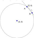
Exercise 3.1.10 Technology. Suppose plasma penicillin concentration in a patient following injection of 1 gram of penicillin is observed to be
P(t) = 200 2
-omt
where t is time in minutes and P(t) is /ig/ml of penicillin. Use the following steps to approximate the rate at which the penicillin level is changing at time t = 5 minutes and at t = 0 minutes.
a. t = 5 minutes. Draw the graph of P(t) vs t for 4.9 <t< 5.1. (The graph should appear to be a straight line on this short interval.)
b. Complete the table on the left, computing the average rates of change of penicillin level.
CHAPTER 3. THE DERIVATIVE
122
c. What is your best estimate of the rate of change of penicillin level at the time t — 5 minutes? Include units in your answer.
d. t = 0 minutes. Complete the second table above. The OMIT entries in the second table refer to the fact that the level of penicillin, P(t), may not be given by the formula for negative values of time, t. What is your best estimate of the rate of change of penicillin level at the time t — 0 minutes?
Exercise 3.1.11 The patient in Exercise 3.1.10 had penicillin level 200 //g/ml at time t — 0 following a 1 gram injection. What is the approximate volume of the patient’s vascular pool? If you wished to maintain the patient’s penicillin level at 200 /xg/ml, at what rate would you continuously infuse the patient with penicillin?
Exercise 3.1.12 Find equations of the lines tangent to the graphs of the function F at the indicated points.
a. F{t) = t 2 at (2,4) b. F(t) = t 2 + 2 at (2,6)
c. F(t) = t + 1 at (2,3) d. F(t) = 3t 3 – At 2 at (1,-1)
e. F(t) = l/(t + l) at (1,1/2) f. F(t) = ^ at (1,1)
Exercise 3.1.13 Find the rates of change of the function F at the indicated points.
a. F(t) = t 3 at (2,8) b. F(t) = 1/t at (2,1/2)
c. F(t) = 2t + t 2 at (2,8) d. F(t) = \/t at (4,2)
e. F(t) = t/(t + l) at (1,1/2) f. F(t) = (t + l)/t at (1,2)
Exercise 3.1.14 In Figure Ex. 3.1.14 is the graph of a parabola with vertex at A and a secant to the parabola through A and a point B What number does the slope of the line containing A and B approach as B approaches Al
Figure for Exercise 3.1.14 A parabola with vertex at A and a secant through A and a point B.
See Exercise 3.1.14.
CHAPTER 3. THE DERIVATIVE
123
3.2 Limit and rate of change as a limit
The phrase
F(b)-F(a)
as b approaches a approaches m a (3.4)
b — a
introduced in the previous section to define slope of a tangent to the graph of F at a point (a, F(a)) can be made more explicit. Almost 200 years after Isaac Newton and Gottfried Leibniz introduced calculus (about 1665), Karl Weierstrass introduced (about 1850) a concise statement of limit that clarifies the phrase. Phrase 3.4 would be rewritten
The limit as b approaches a of — — is m a . (3.5)
o — a
We introduce notation separate from that of the phrase 3.4 because ‘limit’ has application well beyond its use in defining tangents.
Definition 3.2.1 Definition of limit. Suppose G is a function, a is a number, and every open interval that contains a contains a point of the domain of G distinct from a. Also suppose L is a number. The statement that
as x approaches a G(x) approaches L
means that if e is a positive number, there is a positive number 5 such that if x is in the domain of G and 0 < \x — a\ < 5 then \G(x) — L\ < e. This relation is denoted by
lim G(x) = L (3.6) and is read, ‘The limit as x approaches a of G(x) is L.’
The statement that ‘lim G(x) exists’ means that G is a function, a is a number,
x—>a v
and every open interval that contains a contains a number in the domain of G distinct from a, and for some number L, lim G(x) = L.
x—*a
The use of the word ‘limit’ in Definition 3.2.1 is different from its usual use as a bound, as in ‘speed limit’ or in “1. the point, line or edge where something ends or must end; • • •” (Webster’s new College Dictionary, Fourth Edition). Perhaps ‘goal’ (something aimed at or striven for) would be a better word, but we and you have no choice: assume a new and well defined meaning for ‘limit.’
Important. In Definition 3.2.1, the question of whether G(a) is defined is irrelevant, and if G(a) is defined, the value of G(a) is irrelevant. The inequality 0 < \x — a\ < 5 specifically excludes consideration of x — a. Two illustrative examples appear in Figure 3.13. They are the graphs of Fi and F 2 , defined by
, _ f \*x for x ^ 1 , s _ f \x for x ^ 1 , .
1{X) ~ \ not defined for x = l 2[X) ~\ 1 far i = l 1 }
CHAPTER 3. THE DERIVATIVE
124
A
B
Figure 3.13: A. Graphs of F± and F 2 as defined in Equation 3.7.
0.5.
lim Fx(x) = 0.5, and lim F 2 (x)
X— »1 X— >1
5?/ Definition 3.2.1: Suppose e is a positive number; choose 5 = e.
If x is in the domain of F x and 0 < |x — 1| < 5,
1,
then
35
11 1 ,
1\ < -5 < e. 1 2
0.5
The same argument applies to F 2 . That ^(1) = 1 does not change the argument because 0 < \x — 11 < 5 excludes x = 1.
Example 3.2.1 Practice with e’s and 5’s.
1. Suppose administration of a = 3.5 mg of growth hormone produces the optimum serum hormone level L = 8.3 fig in a 24 kg boy. Suppose further that an amount x mg of growth hormone produces serum hormone level G(x) /ig. You may wish to require e = 0.25 fig accuracy in serum hormone levels, and need to know what specification S mg accuracy to require in preparation of the growth hormone to be administered. That is, if the actual amount administered is between 3.5 — 5 mg and 3.5 + 5 mg then the resulting serum hormone level will be between 8.3 — 0.25 = 8.05 fig and 8.3 + 0.15 = 8.45 fig. If instead of e = 0.25 fig, your tolerance is e = 0.05 fig, the specified 5 mg would be smaller.
2. Show that if a is a positive number, then
lim \fx = \fa (3.8) a. Suppose x is in the domain of yfx and 0 < \x — a\ < 5. Then
Suppose e > 0. Let 5 = e \y/x – y/a\ =
X
X
(‘») <
X
{iii) <
S
(iv)
e
(v)
C.
Explore 3.2.1 Our choice of 5 = e -*/a is a bit of a fortuitous lightning bolt 3 , Step (i) is an algebraic trick, you may well wonder why Step (ii) is even correct or not strictly <, you may wonder where 5 came from in Step (Hi), the fortuitous lightning bolt is the reason for Step (iv) and explains why we chose 5 = e ^/a, but by this time you may even doubt Step (v). You would be wise to check each step, h
CHAPTER 3. THE DERIVATIVE
125
3. Find a number 5 > 0 so that
if 0<|x-l|<5
then
1 + x 2
0.5
< 0.01.
A graph of y = 1/(1 + x 2 ) is shown in Figure 3.14 along with lines a distance 0.01 above and below y = 0.5. We solve for x at the intersections of the lines with the graph.
= 0.49, x = 1.0202;
1 + x
From the graph it is clear that
and
1 + x
2 = 0.51,
x = 0.98019.
if 0.981 < x < 1.02 then 0.49 < We choose 5 = 0.019, the smaller of 1.0 – 0.981 and 1.02 – 1.0.
Thru if 0 < \x – II < 6, — 7t – 0.5
1 + x’
< 0.51.
1 + x 2
< 0.01.
A
B
0 0.2 0.4 0.6 0.8
0.85 0.9 0.95
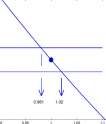
Figure 3.14: A. Graph of F(x) = 1/(1 + x 2 ), and B a magnification of A. In both graphs, segments of the lines y = 0.49 and y = 0.51 are drawn.
4. Find a number 6 > 0 so that
if 0 < \x – 41 < 5
then
1 1
~x ~ 2
x – 4 + 16
< 0.01.
This algebraic challenge springs from the problem of showing that the slope of
f(x)
at the point (4,-) is —. x 2 16
We first do some algebra.
1 1
x 2 1 +
2-y/X
2Jx
x-4 16
x
+
-8 + ^(^ + 2) 2)(v^ + 2) ‘ 16^2^(^ + 2) ‘ 16 ~ 16^(^ + 2)
•1 1
+
CHAPTER 3. THE DERIVATIVE
126
It is sufficient to find 5 > 0 so that
if 0 < \x – 41 < 5 then
-8 + ^(^ + 2)
16^(v^ + 2)
< 0.01 or
-8 + ^(^ + 2)
< 0.16
Assume that x is ‘close to’ 4 and certainly bigger than 1 so that the denominator, y/x{^/x + 2) is greater than I. Then it is sufficient to find 5 > 0 so that
-8 + x + 2 v ^x
< 0.16.
-8 + ^(^ + 2) = Let z = y/x so that z 2 = x and solve
-8 + z 2 + 2z = -0.16 and -8 + z 2 + 2z = 0.16
Zl
1.97321
Z2
2.026551.97321
xi = 3.89356 We will choose 5 — 0.1 so that
x 2 = 4.10690
if 0 < \x — 41 < 0.1 then x is between x\ and x 2 and
1 1
7^~2 1 x – 4 16
< 0.01.
5. Suppose you try to ‘square the circle.’ That is, suppose you try to construct a square the area of which is exactly the area, ir, of a circle of radius 1. A famous problem from antiquity is whether one can construct such a square using only a straight edge and a compass. The answer is no. But can you get close?
Suppose you will be satisfied if the area of your square is within 0.01 of ir (think, e = 0.01). It helps to know that
7T = 3.14159265—, and 1.77 2 = 3.1329,
and that every interval of rational length (for example, 1.77) can be constructed with straight edge and compass. Because 1.77 2 = 3.1329 is within 0.01 of 7r, you can ‘almost’ square the circle with straight edge and compass.
Explore 3.2.2 Suppose you are only satisfied if the area of your square is within 0.001 of n. What length should the edges of your square be in order to achieve that accuracy? ■
Now suppose e is a positive number and ask, how close (think, 5) must your edge be to y/n in order to insure that
the area of your square — n
<
Let x be the length of the side of your square. Your problem is to find S so that
if \x — < 5, then \x — ir\ < e. Danger: This may fry your brain. Look at the target \x 2 — ir\ < e and write
\x — 7T < e
\x
Lets require first of all that 0 < x < 5. (We get to write the specifications for x.) Then
x + v^r < 10. (Actually, -Jix = 1.7725 so that x + y/n is less than 7, but we can be generous.) Now
look at our target,
\x 2 — 7r| = \x — \fii\ \x + y/n\ < e Choose 5: Insist that \x — < 5=Minimum(e/10,1). Then 0 < x < 5, and
\x 2 — 7r| = |x — |x + \Ztt\ < — ■ 10 = e.
If |x — < 5 = Minimum(e/10,1), then \x 2 — n\ < e.
Explore 3.2.3 We required that 0 < x < 5. (We get to write the specifications for x.) Would it work to require that 0 < x < 1? ■
Using the definition of limit we rewrite the definitions of tangent to the graph of a function and the rate of change of a function.
Definition 3.2.2 Definition of tangent and rate of change, revisited.
Suppose F is a function, a is a number in the domain of F, and every open interval that contains a contains a point of the domain of F distinct from a, and m a is a number. The statement that the slope of the tangent to the graph of F at (a, F(a)) is m a and that the rate of change of F at a is m a means that
lim
F(b) – F(a) b — a
(3.9)
In the previous section we found that the slope of the tangent to the graph of F(t) = t 2 at a point (a, a 2 ) was 2a. Using the limit notation we would write that development as
lim
b— >a
F(b) ~ F{a) b — a
lim —
b-^a b — a
= lim
b^a
(b – a) (6 + a)
lim (6 + a)
b^a
a + a = 2a
There is some algebra of the limit symbol, lim, that is important. Suppose each of F\ and F 2 is
x—>a
a function and a is a number and \\mFAx) and lim F 2 (x) both exist. Suppose further that C is a number. Then
CHAPTER 3. THE DERIVATIVE
128
Probably all of these equations are sufficiently intuitive that proofs of them seem superfluous. Equations 3.10 and 3.11 could be more accurately expressed. For Equation 3.10 one might say,
“If FAx) = Cfor all a then lim F^x) = C.” (3.16)
x—>a
Explore 3.2.4 Suppose F\ is defined by
Fi(ar) = C if x^a
Fx (a) = C+l
Is it true that
lim FAx) = C ?
x^a
Explore 3.2.5 Write a more accurate expression for Equation 3.11 similar to the more accurate expression 3.16 for 3.10. ■
Proof of Equations 3.12, 3.13 and 3.14 are rather easy and are included to illustrate the process. Proof of Equation 3.12. Suppose a^0 and e > 0. Let
5 = Minimum(|a|/2, e a 2 /2). Suppose 0 < \x — a\ < 5.
Note: Because \x — a\ < 5 < \a\/2, \x\ > \a\/2 and \x a\ > \a 2 \/2.
Proof of Equation 3.13. Let lim Fi(x) = L\. Suppose e is a positive number. Case C — 0. Let 5 — 1. Then if x is in the domain of F\ and 0 < \x — a\ < S,
\CF 1 {x) -CLi\ = |0-0| = 0 < e.
Case C ^ 0. Let
€o = W\
Because lim FAx) = L±, there is S > 0 such that if 0 < \x — a\ < 5 then \Fi(x) — L\\ < e 0 . Then if
x^a
x is in the domain of F and 0 < \x — a\ < S,
\CF x {x) – CLi| = |C| |Fi(a;) – L ± \ < \C\ e 0 = \C\-^- = e.
\C |
Thus
lim CFAx) = C L x = C lim FAx) Proof of Equation 3.14. Suppose lim FAx) = L\ and lim FAx) = L 2 . Suppose e > 0. There are
x^a x^a
numbers Si and 5 2 such that
if 0 < \x — a\ < Si thenlF^rr) — L x \ < ^ and if 0 < \x — a\ < S 2 then|F 2 (x) — L 2 \ < ^
Let S = Minimum (Si, S 2 ). Suppose 0 < \x — a\ < S. Then
\Fi(x) + F 2 (x)-(Li + L 2 )\ < \Fi(x)-Li\ + \F 2 (x)-L 2 \
e e < 2 + 2 =f
Honest Exposition. Almost always in evaluating
lim F(x),
x^a
if F is a familiar function and F(a) is defined then
lim Fix) = F(a).
x— >a
If this happens, F is said to be continuous at a (more about continuity later). It follows from Equations 3.10 through 3.15, for example, that
if P(x) is any polynomial, then lim P(x) = P(a). See Exercise 3.2.7.
Moreover, even if F(a) is not meaningful but there is an expression E(x) for which
F(x) = E(x) for x 7^ a, and E(a) is defined,
then almost always
lim Fix) = Eia).
x—>a
For example, for
x 4 _ a 4
Fix) = , Fia) is meaningless.
x — a
CHAPTER 3. THE DERIVATIVE
130
But,
for x 7^ a, F(x)
(x – a)(x 3 + ax 2 + a 2 x + a 3 )
x — a
= x 3 + x 2 a + x a 2 + a 3
= E(x).
and E(a) = 4a 3 , and Inn F(x) = 4a 3 . The simple procedure just discussed fails when considering more complex limits such as
SIM
lim
x~*0 x
lim , and lim .
x->i rr — 1 x-t-i x — 1
Limit of the composition of two functions. A formula for the limit of the composition of two functions has very broad application.
Suppose u is a function, L is a number, a is in the domain of u, and there is an open interval (p, q) in the domain of u that contains a and if x is in (p, q) and is not a then u(x) ^ L. Suppose further that
lim u(x) = L
Suppose F is a function and for x in (p, q), u{x) is in the domain of F, and
Then
lim F(s) = X.
lim F(u(x)) = A
(3.17)
Intuitively, if x is close to but distinct from a, then u(x) is close to but distinct from L and F(u(x)) is close to A. The formal argument is perhaps easier than the statement of the property, but is omitted.
Some formulas that follow from Equation 3.17 and previous formulas include
If lim F(x) = L > 0, then
x—*a
If lim Fix) = L ^ 0, then
x—>a
If lim F 2 (x) ^ 0, then
lim J Fix) = VL.
1 1
lim .
x^a F[x)
lim ™
lim Fi(x)
(3.18)
Exercises for Section 3.2, Limit and rate of change as a limit.
CHAPTER 3. THE DERIVATIVE
131
Exercise 3.2.1
a. Find a number, 5 > 0, so that if a; is a number and 0 < \x — 2| < 5 then \2x — 4| < 0.01.
b. Find a number, 5, so that if x is a number and 0 < |x — 2\ < 5 then
c. Find a number, 5, so that if a; is a number and 0 < \x — 2| < 5 then
d. Find a number, 5, so that if a; is a number and 0 < \x — 2| < 5 then
e. Find a number, 5, so that if x is a number and 0 < \x — 2| < 5 then
f. Find a number, <5 > 0, so that if x is a number and 0 < \x — 9| < 5 then (a/x — 3| < 0.01.
g. Find a number, 5, so that if a; is a number and 0 < \x — 8| < 8 then \^fx — 2| < 0.01.
h. Find a number, 5 > 0, so that if a; is a number and 0 < \x — 2| < 5 then la; 4 -3a;- 131 < 0.01.
Exercise 3.2.2 a. Find a number, 5 > 0, so that
if x is a number and |rr — 3| < 5 then
b. Find a number, <5 > 0, so that
if a; is a number and \x — 4| < 5 then
c. Find a number, 5 > 0, so that
if x is a number and \x — 2| < 5 then
d. Find a number, <5 > 0, so that
if x is a number and |rr — 1| < 5 then Exercise 3.2.3 a. Use Equations 3.11 and 3.15,
x 2 -9 x — 3
-6
< 0.01.
v^-2 1 x – 4 4
< 0.01.
1 1
a; ~ 2 x – 2
+
< 0.01.
x 2 + x – 2 x – 1
< 0.01.
lim x = a and lim Fi{x) x F 2 (x) = ( lim F\{x) I x l lim P2{x) ) ,
( lim F 2
to show that
b. Show that
c. Show by induction that if n is a positive integer,
lim x 2 = a 2 .
x^a
lim x 3 = a 3 .
x^a
lim x n = a n .
x^a
(3.19)
CHAPTER 3. THE DERIVATIVE
132
Exercise 3.2.4 Prove the following theorem.
Theorem 3.2.1 : Limit is Unique Theorem. Suppose G is a function and
lim G(x) = Li and lim G(x) = L 2 .
x—>a x^a
Then L 1 = L 2 .
Begin your proof with,
1. Suppose that L\ < L 2 .
2. Let e = (L 2 – U)/2.
Exercise 3.2.5 Evaluate the limits.
a. lim 3x 2 — 15a; b. lim 3a; c. lim n
x-^5 x~*0 x— >50
d. lim 3a; 2 — 15a; e. lim x f. lim 50
x — 1 x 2 — 2a; + 1 x 4 — 1 g. hm h. hm l. lim
x->-5 x — 1 x->l x — 1 x->l x — 1
^ / 1£ 2 I oc 3
j. lim = k. lim \ —s 1. lim
x^a ^ x + 2x 2 z-iyV + i ‘ ^iv^ 3 -27
Exercise 3.2.6 Sketch the graph of y = \fx for — 1 < x < 1. Does the graph have a tangent at (0,0)? Remember, Your vote counts.
Exercise 3.2.7 Suppose P(x) = a n x n + a n ^\x n ~ x + • • • a\x + ao is a polynomial and a is a number. For each step {%) through (vii), identify the equation of Equations 3.10 – 3.14 and 3.19 that justify the step.
lim P(x) = lim \a n x n + a n _\X n ~ x + • • • a\X + a 0 )
x^a x^a \ J
= lim (a n x n ) + lim ( a n -\x n ~ l + ■ ■ ■ a±x + a 0 ) (i)
x—*a x^a \ J
= lim (a n x n ) + lim {a n -\x n ~ l ) + lim ( a n -2X n ~ 2 ■ ■ ■ a±x + ao) (ii)
x^a x^a \ / x^a \ /
= lim (a n x n ) + ■ ■ ■ + lim (a 2 x 2 ) + lim (a\x + a 0 )
= lim (a n x n ) + ■ ■ ■ + lim (c^a; 2 ) + lim (aix) + lim (a 0 ) (w)
x—>a x—+a \ / x^a x^a
= a n lim (x n ) + • • • + a 2 lim (x 2 ) + a\ lim (x) + lim (ao) (iv)
x-^a x^a \ / x^a x^a
= a n a n + ■ ■ ■ + a 2 a 2 + a\ lim (x) + lim (ao) (v)
x—>a x^a
= a n a n + a n _ia n_1 + • • • + a 2 a 2 + a x a + lim (a 0 ) (wi)
= a„a™ + a n -\a n ~ l + • • • + 02a 2 + aia + ao (vii) = P(a) Whew!
CHAPTER 3. THE DERIVATIVE
133
Exercise 3.2.8 . Show that Equation 3.13,
lim C FAx) = C (\im Fx(x”
x^a \x^a ‘
follows from Equations 3.10 and 3.15,
lim C = C and lim (FAx) F 2 (x)) = f lim FAx) ) (lim F 2 (x’
x~*a x—>a \ x-^a J \x—hi ‘
Exercise 3.2.9 Some of the following statements are true and some are false. For those that are true, provide proofs using Equations 3.10 – 3.15. For those that are false, provide functions Fi and F 2 to show that they are false. Assume the limits shown do exist. Suppose Fi and F 2 are functions defined for all numbers, x.
Exercise 3.2.11 Suppose F(x) is a function and
lun Fm-F(2)
b^2 b-2
exists.
What is lim F(b) ?
CHAPTER 3. THE DERIVATIVE
3.3 The derivative function, F’
134
Definition 3.3.1 The function, F’. Suppose F is a function and for some number, x, in its domain the rate of change of F exists at x. Then the function F’ (read ‘F prime’) is defined by
F\x) = the rate of change of F at x (3.20)
for all numbers x in the domain of F for which the rate of change of F at x exists.
Equivalently,
F'(x) = the slope of the graph of F at ( x, F(x) ) (3-21)
for points ( x, F(x)) of the graph of F for which the tangent exists. Symbolically, we may write
n*) = ** m r F(x) . (3.22)
V ‘ b^x b-x
The function F’ is called the derivative 4 ” of F (the function derived from F). When the independent variable of F is expressed as in F(x), F'(x) is the derivative of F(x) with respect to x.
The derivative is one-half of calculus, perhaps 4 percent of your university education, and requires your attention. The next 200? pages of this text present biological and physical interpretations of the derivative, formulas for computing the derivatives of commonly encountered functions, and uses of derivatives in writing equations for mathematical models of biological and physical systems.
Example 3.3.1 You found in Chapter 1, Problem 1.9.1 on page 45 that light intensity, L, at a distance, d, from a linear slit of light was
1 45
L(d) = —— 3 < d < 16
(Jj
where L was measured in mW/cm 2 and d was measured in cm.
4 Joscph-Louis Lagrange (a French mathematician of Italian descent, 1736-1813) used the word ‘derivative’, and may have been the first to do so (H. L. Vacher, Computational geology 5 – If geology, then calculus, J. Geosci. Educ, 1999, 47 186-195).
CHAPTER 3. THE DERIVATIVE
135
At what rate is the light decreasing when d = 5 cm? We find the derivative of L. For any value of d between 3 and 16 cm,
L\d) = lim
6—>d
= lim
L(b) – L(d) mW/cm 2 b — d cm
1.45 1.45
mW/cm 2
cm
/ , 1 \ mW/cm 2 hm -1.45 4
cm
-1.45 mW/cm 2
For d = 5, L'(5)
rf 2
-1.45
cm
d 2
■1.45
-0.058
d=5
We have just used a helpful notation:
mW/cm 2
cm

It is useful to compare the algebraic forms of L and L’,
k 1 1
L(d) — – and L'(d) =—k—^, and note that L'(d) = — -L 2 (d). & & K
Explore 3.3.1 For one mole of oxygen at 300° Kelvin the pressure, P in atmospheres, and volume, V in liters, are related by
„ 1 x 0.0820 x 300
V
a. Find the derivative of P with respect to V.
b. What is P'(l)?
The question of units on the rate of change is important. We have used the following.
CHAPTER 3. THE DERIVATIVE
136
Units on F’
If lim G(x) = L
x— >a
then the units on L are the units on G.
It follows that the units on
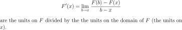
• If F(t) is distance in meters and t is time in seconds, then F'(t) is meters per second, or velocity.
• If F(x) is pressure in atmospheres and x is altitude in km, then F'(x) is commonly called the pressure gradient and is measured in atm/km.
• If F(t) is population size in individuals and t is time in years, then F'(t) is population growth rate (which might be negative) in individuals per year.
It is useful to see the rate of change of F over the whole domain of F. In Figure 3.15A is the graph of a function, called a logistic function, that is typical of the size of population that starts at low density and grows in a limited environment. At time t — 0 the population size is P(0) = 1 and the maximum supportable population is M = 10. Its derivative is shown in 3.15B and illustrates population growth rate. The maximum of the derivative occurs at t = 3.17 and this marks the steepest part of the population graph. The growth rate initially is low, rises to a maximum at t = 3.17, and decreases again as population density nears its maximum.
A
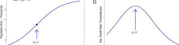
Max Pop = 10
Time – Years
Time – Years
Figure 3.15: A. Graph of a classical logistic curve, L, describing population size as a function of time. B. A graph of L’, the population growth rate.
CHAPTER 3. THE DERIVATIVE
137
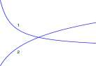
Figure 3.16: The graph of a function P and its derivative P’.
Example 3.3.2 Problem. The graphs of a function P and its derivative P’ are shown in Figure 3.16. Which graph is the graph of PI
Solution. We claim that graph 1 is not P, because every tangent to graph 1 has negative slope and some y-coordinates of graph 2 are positive. Therefore graph 2 must be the graph of P.
Alternate notation. Calculus originated in England with Sir Isaac Newton (1642-1727) and in Germany with Gottfried Wilhelm Leibniz (1646-1716), and indeed some elements of it were anticipated by the Greek mathematicians. Given the multiple origins and a 300 year history, it is not surprising that there are several notations for derivative. Newton used y’ for the ‘fluxion’ of y (rate of change of y). But when the independent variable was time, Newton used the symbol y for the rate of change of y and y for the second derivative of y (the derivative of the derivative of y). Therefore if y denotes distance, y denotes velocity and y denotes acceleration. The most common notation, for the derivative was introduced and used by Leibnitz. When discussing the rate of change of F at a number a one may see
F’ia)
or
dF
dx
or
dF
dx
or
F
or
F(a)
A function that has a derivative is called a differentiable function. To differentiate F means to compute the derivative, F’. “Differentiable” comes from the concept of a ‘differential’ which is a cousin of an elusive concept called ‘infinitesimal’. An infinitesimal is a positive number that is less than all other positive numbers, which is possible only in an extension of our familiar number system. An infinitesimal change, dx, in x causes an infinitesimal change, dF, in F(x) and the derivative is the ratio 4^. The concept of a limit is considered to be less mysterious than is infinitesimal, and can easily be put on a quite sound footing, whereas it is difficult to define ‘infinitesimal’ clearly 5 .
It is sometimes preferable to substitute h for b — x so that b = x + h, and write
F'(x)
lim
b— >x
F(b) – F(x) b — x
as
F'(x)
lim
h-fO
F(x + h) -F(x) h
(3.23)
5 Abraham Robinson, Nonstandard Analysis, Princeton University Press, 1996 is a recent book defining calculus based on infinitesimals.
CHAPTER 3. THE DERIVATIVE
Exercises for Section 3.3, The derivative function, F’. Exercise 3.3.1 Use Equation 3.22,
F(b) – F(x)
F'(x) = lim
b^x
b — x
to compute F'(x) for
Exercise 3.3.2 Use the equation,
% , F(x + h) -F(x) F (x) = lim
to comupute F'(x) for: a. F(x)
d. F(x)
x
X
b. F{x) F(x)
c.
h
3x 2 2X1
c. F(x) f. F(x)
x 2 + 5 x1 -7
Exercise 3.3.3 In Figure Ex. 3.3.3A and Figure Ex. 3.3.3B are four pairs of graphs of a function P and and its derivative, P’. For each pair, which is the graph of PI Explain your choice.
Figure for Exercise 3.3.3 A. Graphs of a function and its derivative for Exercise 3.3.3.
CHAPTER 3. THE DERIVATIVE 139 Figure for Exercise 3.3.3 B. Graphs of a function and its derivative for Exercise 3.3.3.
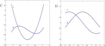
Exercise 3.3.4 a. In Exercise Figure 3.3.4A is the graph of a function, F. Estimate the slopes of the tangents to that graph at the points marked on the graph. Plot a new graph of slopes vs the dependent variable for F. Sketch a graph of F’.
b. Repeat the steps of the part a. for the graph of a function, G, in Exercise Figure 3.3.4B.
Figure for Exercise 3.3.4 A. Graph of a function F for Exercise 3.3.4a. B. Graph of a function
G for Exercise 3.3.4b.
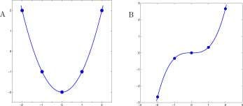
Exercise 3.3.5 Danger: Obnubilation Zone.
a. Shown in Exercise Figure 3.3.5A is a graph of the derivative, F’, of a function, F. One point of the graph of F is (0,2) (that is, F(0) = 2). Your job, should you accept it, is to sketch a reasonable graph of F.
b. Repeat the steps of a. to sketch a graph of a function G knowing that G(l) = 0 and the graph of G'(x) is shown in Exercise Figure 3.3.5B. (Consider: What is the slope of G at x = 1? What is the slope of G at x = 2? What is the slope of G at x = 3?)
Figure for Exercise 3.3.5 A. Graph of F’ for a function F for Exercise 3.3.5a. B. Graph of G’
for a function G for Exercise 3.3.5b.
CHAPTER 3. THE DERIVATIVE
140
A 2
B
0 –

Exercise 3.3.6 In Figure 3.15A it appears that at t = 6 years the population was about 8.75 thousand, or 8,750 individuals and that the growth rate was about 0.75 thousand per year, or 750 individuals per year. Suppose this is a deer population and you wished to allow hunters to harvest some deer each year. How many deer could be harvested each year and the population size remain at 8,750 individuals?
Exercise 3.3.7 Technology. The function
is an example of a logistic function, a type of function that often is used to describe the growth of populations. Plot the graph of this function for 0 < t < 10, 0 < y < 20. Find how to plot P'(t) and locate the highest point of P'(t) on your technology. MATLAB code is
close all;clc;clear; h=0.001; x=[0:h:5]; y=10./(9*2.”(-x)+1);
z=diff(y)/h; [m,i]=max(z); [x(i) y(i) z(i)]
plot(x,y,’linewidth’ , 2); hold(‘on’)
plot(x(i),y(i),’x’ , ‘linewidth 5 ,3)
plot(x(l:length(x)-l),z,’r’ ,’linewidth’,2)
plot(x(i),z(i),’xr’,’linewidth’,3)
At what time and population size is the population growing the fastest?
Exercise 3.3.8 The square function, S(t) = t 2 , t > 0, and the square root function, R(t) = y/t, t>0, are each inverses of the other. See Figure Ex. 3.3.8. Compare the slopes of the tangents to S at the points (2,4), (3,9), and (4,16) with the slopes of R at the respectively corresponding points, (4,2), (9,3), and (16,4) of R. Compare the slope of the graph of S at the point (a, a 2 ), a > 0 with the slope of the graph of R at the corresponding point (a 2 , a).
P(t)
10 2*
10
9 + 2*
(9 2~* + l)
CHAPTER 3. THE DERIVATIVE
141
18 16 14 12 10
8
6
4
2
0
The next two exercises explore the reflective property of a parabola which asserts that light rays originating from the focal point of a parabola will strike the parabola and be reflected in a direction parallel to the axis of the parabola. We choose the parabola that is the graph of y = 2\/t which has (1,0) as its focal point and x = —1 as its directrix.
Figure 3.17: A parabolic reflector used to boil water in the kettle that is at the focal point of the dish, in Lhasa, Tibet.
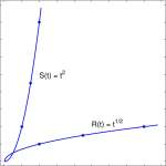
Exercise 3.3.9 Shown in Figure Ex. 3.3.9 is the graph of y = 2yi and a ray emanating vertically from the focal point at (1,0) and reflected (apparently horizontally) by the tangent to the parabola at (1,2). The angles A (of incidence) and B (of reflection) are equal.
a. Compute the slope of the tangent to y = 2y/i at the point (1,2).
b. Argue that the angle A in Figure Ex. 3.3.9 is 45°.
c. Argue that the angle B in Figure Ex. 3.3.9 is 45°.
d. Argue that the reflected ray from (1,2) is horizontal.
Figure for Exercise 3.3.9 Graph of the parabola y = 2\ft and a ray (dashed line) emanating vertically from the focal point (1,0) and reflected at (1,2). See Exercise 3.3.9.
CHAPTER 3. THE DERIVATIVE
142
Exercise 3.3.10 Shown in Figure Ex. 3.3.10 is the graph of y = 2\^i, and a ray (dashed line) from the focal point, (1,0), to the point (a, 2-^/a), and a tangent, T, to the parabola at (a, 2-^/a). Our goal is to show that the reflected ray (dashed line with arrow head) is horizontal (but it has not been drawn that way). The two angles marked (3 are equal because they are vertical angles of intersecting lines.
It will be sufficient to show that the angle of reflection, B, is also (3, the angle of inclination of the tangent T. Because B and (3 are acute, it will be sufficient to show that tan B = tan (3.
a. Argue that C = A + (3, so that A = C – (3.
b. Argue that B = A, so that B = C – (3.
c. Compute the slope of the tangent T to the graph of y = 2y/t at (a, 2y/a). By definition, this number is also tan (3.
d. Compute tanC.
e. Use the trigonometric identity
tan(C – (3)
tan C — tan (3
1 + tan C tan (3 to show that t&nB = tan(C — 0) — 4g. Because tan B = tan (3, B = (3 and the reflected ray is horizontal.
Figure for Exercise 3.3.10 Graph of the parabola y = 2y/i and a ray (dashed line) emanating vertically from the focal point (1,0) and reflected at a point (a, 2-y/a). See Exercise 3.3.10.
CHAPTER 3. THE DERIVATIVE
143
2 –
1 –
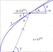
0.5
1 1.5
2.5
3.5
3.4
Mathematical models using the derivative.
The rate of change of a function provides a powerful new way of thinking about models of biological processes.
The changes in biological and physical properties that were measured in discrete packages (Pt+i — Pt, A t +\ — A t , J t+1 — /() in Chapter 1 can be more accurately represented as instantaneous rates of change (P'(t), A'(t), I'(t)) using the derivative. In Section 1.1, Table 1.1, the V. natriegens population was measured at 16 minute intervals but was growing continuously. The kidneys filter continuously, not in 5-minute spurts. Here we begin a process of using the derivative to interpret mathematical models that continues through out the book.
We wrote in Section 1.5 that the daily increase in the area of a mold colony is proportional to the circumference of the colony at the beginning of the day. Alternatively, we might say:
Mathematical Model 3.4.1 Mold growth. The rate of increase in the area of the mold colony at time t is proportional to the circumference of the colony at time t.
Letting A(t) be area and C(t) be circumference of the mold colony at time t, we would write
3.4.1
Mold growth.
A'(t) = k C(t)
Because C(t) = JA(t) (assuming the colony is circular)

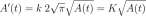
(3.24)
where K = k
CHAPTER 3. THE DERIVATIVE
144
Equation 3.24, A'{t) = KJA(t), is a statement about the function A. We recall also that the area of the colony on day 0 was 4 mm 2 . Now we search for a function A such that
A{0) = 4 A'(t) = KyjA{t) t > 0 (3.25)
Warning: Incoming Lightning Bolt. Methodical ways to search for functions satisfying conditions such as Equations 3.25 are described in Chapter 17. At this stage we only write that the function
Ait) = (— t + 2 J t>0 Bolt Out of Chapter 17. (3.26)
satisfies Equations 3.25 and is the only such function. In Exercise 3.6.7 you are asked to confirm that A(t) of Equation 3.26 is a solution to Equation 3.25.
Finally, we use an additional data point, A{8) = 266 to find an estimate of K in A(t) = (ft + 2) 2 .
A(8) = (y 8 + 2 ) 266 = (4K + 2) 2
2
K
3.58
Therefore, A(t) = (1.79t + 2) describes the area of the mold colony for times 0 < t < 9. Furthermore, A has a quadratic expression as suggested in Section 1.5 based on a discrete model. A graph of the original data and A appears in Figure 3.18.
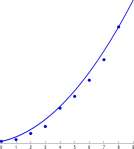
2 3 4 5
Time – days
Figure 3.18: Graph of A(t) = (1.79£ + 2 ) 2 and the area of a mold colony from Table 1.5
3.4.2 Difference Equations and Differential Equations.
We have just seen our first example of a differential equation, Equation 3.24. It writes the derivative, A'(t), of a function in terms of the function, = K J A(t). We prefer the term derivative
CHAPTER 3. THE DERIVATIVE
145
equation but defer to the almost universal use of differential equation. The comparison is
A t+l -A t = K^A A 0 = 4 A'(t) = KA(t) A(0) = 4
vs
Difference Equation Differential Equation
Differential equations often more accurately represent the biological, physical chemical, economic, or social system under study because the equation and solution are defined throughout a time interval or space interval, whereas difference equations and solutions are defined only for discrete sequences of numbers, and maybe a finite sequence. Deer populations that breed only annually, however, may be better represented by a difference equation
Difference equations are inherently simpler than differential equations. Solutions to difference equations require only arithmetic, whereas solutions to differential equations involve calculus. The solution to the difference equation above seems to only have an arithmetically derived solution. The corresponding differential equation has a simple algebraic solution, t + . You have to wait 14 chapters before we describe its derivation, but we will write and solve differential equations in Chapters 5, 7 and 13.
Some computers will return solutions to differential equations, much as looking up addresses in a telephone book. Give ‘White Pages’ on the internet a name and area code, and it will return the address, telephone number, age and close associates of a person, and perhaps another one or two people, with that name and area code. Computers are very adept, however, at computing approximate solutions to some very complex differential equations, such as those that describe the path of a manned space craft traveling to the moon. Ironically, what they actually do is compute solutions to difference equations closely associated with the a differential equation; computers are arithmetic whizzes.
3.4.3 Chemical kintetics.
Chemists use the rate of change in the amount of product from a chemical reaction as a measure of the reaction rate. You will compute some rates of chemical reactions from discrete data of chemical concentration vs time.
Chemical reactions in which one combination of chemicals changes to another are fundamental to the study of chemistry. It is important to know how rapidly the reactions occur, and to know what factors affect the rate of reaction. A reaction may occur rapidly as in an explosive mixture of chemicals or slowly, as when iron oxidizes on cars in a junk yard. Temperature and concentration of reactants often affect the reaction rate; other chemicals called catalysts may increase reaction rates; in many biological processes, there are enzymes that regulate the rate of a reaction. Consider
A— >B
to represent (part of) a reaction in which a reactant, A, changes to a product, B. The rate of the reaction may be measured as the rate of disappearance of A or the rate of appearance of B.
CHAPTER 3. THE DERIVATIVE
146
-20 0 20 40 60 80 100 120 140 160
Time sec
Figure 3.19: Conductivity of a water and butyl chloride solution at times after butyl chloride was added to water.
Butyl chloride.
When butyl chloride, C 4 H 9 C1, is placed in water, the products are butyl alcohol and hydrochloric acid. The reaction is
C 4 H 9 C1 + H 2 0 —> C 4 H 9 OH + H + + CP
As it takes one molecule of C4H9CI to produce one atom of CI , the rate at which butyl chloride disappears is the same as the rate at which hydrochloric acids appears. The presence of CI” may be measured by the conductivity of the solution. Two students measured the conductivity of a solution after butyl chloride was added to water, and obtained the results shown in Figure 3.19. The conductivity probe was calibrated with 8.56 mmol NaCl, and conductivity in the butyl chloride experiment was converted to mmol CI . The experiment began with butyl chloride being added to water to yield 9.6 mmol butyl chloride.
The average rate of change over the time interval [30,40]
1.089 – 0.762 m30,4 ° = — 4o_30 — = °0327 ‘
and the average rate of change over the time interval [40,50]
1.413-1.089 m 40,so = _ n . n = 0.0324. 50 — 40
both approximate the reaction rate. A better estimate is the average of these two numbers, 0.0327+0.0324 _ q. 03255. We only use the average when the backward and forward time increments, -10 seconds and +10 seconds, are of the same magnitude. The average can be computed without computing either of the backward or forward average rates, as
1.413 – 0.762
w-30,50 = —~—™— = 0.03255 50 — 30
In the case of t — 150, knowledge of the forward time increment is not available, and we use the backward time increment only.
3.355 – 3.255 n M
CHAPTER 3. THE DERIVATIVE
147
Explore 3.4.1 Estimate the reaction rate at time t = 80 seconds. ■
Example 3.4.1 It is useful to plot the reaction rate vs the concentration of CI – as shown in Figure 3.20. The computed reaction rates for times t = 0, 10, • • • 40 are less than we expected. At these times, the butyl chloride concentrations are highest and we expect the reaction rates to also be highest. Indeed, we expect the rate of the reaction to be proportional to the butyl chloride concentration. If so then the relation between reaction rate and Cl~ concentration should be linear, as in the parts corresponding to times t = 60, 70, ■ • • 160 s. The line in Figure 3.20 has equation y = 0.0524 — 0.0127x. We can not explain the low rate of appearance of Cl~ at this time.
Figure 3.20: Rate at which CL accumulates as a function of CL~ is added to water.

Concentration C! ([ CP ] | mmol
concentration after butyl chloride
The reaction is not quite so simple as represented, for if butyl alcohol is placed in hydrochloric acid, butylchloride and water are produced. You may see from the data that the molarity of CI – is tapering off and indeed later measurements showed a maximum Cl _ concentration of 3.9 mmol. If all of the butyl chloride decomposed, the maximum Cl~ concentration would be 9.6, the same as the initial concentration of butyl chloride. There is a reverse reaction and the total reaction may be represented
ki
C 4 H 9 Cl(aq) + H 2 0 (1) ^ C 4 H 9 OH(aq) + H+ + CI” (aq)
k 2
The numbers, ki and h%, are called rate constants of the reaction. The number k± is the negative of the slope of the line computed in Example 3.4.1 (that is, 0.0127).
Exercises for Section 3.4 Mathematical models using the derivative.
Exercise 3.4.1 Write a derivative equation that describes the following model of mold growth.
Mathematical Model. A mold colony is growing in a circular pattern. The radius of the colony is increasing at a constant rate.
Exercise 3.4.2 Write a derivative equation that describes the following model of light depletion below the surface of a lake.
Mathematical Model. The rate at which light intensity decreases at any depth is proportional to the intensity at that depth.
Exercise 3.4.3 Write a derivative equation that describes the following model of penicillin clearance.
Mathematical Model. The rate at which the kidneys remove penicillin is proportional to the concentration of penicillin.
Exercise 3.4.4 Data from Michael Blaber of Florida State University College of Medicine 6 for the butyl chloride experiment
C 4 H 9 Cl(aq) + H 2 0(1) -> C 4 H 9 OH(aq) + HCl(aq)
are shown in Table 3.4.4. These are more nearly what one would expect from this experiment.
a. Graph the data.
b. Estimate the rate of change of the concentration of C 4 H 9 C1 for each of the times shown.
c. Draw a graph of the rate of reaction versus concentration of C4H9CI.
Table for Exercise 3.4.4 Data for Ex. 3.4.4.
Exercise 3.4.5 Data from Purdue University for the decrease of the titration marker phenolphthalein (Hln) in the presence of excess base are shown in Table 3.4.5. The data show the concentration of phenolphthalein that was initially at 0.005 M in a solution with 0.61 M OH – ion.
a. Graph the data.
b. Estimate the rate of change of the concentration of phenolphthalein (Hln) for each of the times shown.
c. Draw a graph of the rate of reaction versus concentration of phenolphthalein.
Table for Exercise 3.4.5 Data for Ex. 3.4.5.
Exercise 3.4.6 Data from Michael J. Mombourquette, Queens University, Kingston, Ontario, Canada 8 for the decrease of CO in the reaction
CO(g) + N0 2 (g) – C0 2 (g) + NO (g)
are shown in Table 3.4.6A. and the decrease of N 2 0 5 in the reaction
6 http: / / wind .sb.fsu.edu/cheml046/ notes/Kinetics/Rxnrates.htm 7 http://chcmcd. chcm.purdue.edu/genchem/topicreview/bp/ch22/rate. html
8 http://www.chem.queensu.ca/peoplc/fa...tics/index.htm
CHAPTER 3. THE DERIVATIVE
149
2N 2 0 5 (g) – 4N0 2 (g) +0 2
are shown in Table 3.4.6B. Initially, 0.1 g/1 of CO was mixed with 0.1 g/1 of N0 2 . For each table,
a. Graph the data.
b. Estimate the rate of change of the concentration of CO or of N 2 Os for each of the times shown.
c. Draw a graph of the rate of reaction versus concentration of reactant.
Table for Exercise 3.4.6 Data for Ex. 3.4.6.
A.
B.
3.5 Derivatives of Polynomials, Sum and Constant Factor Rules
We begin a common strategy to find derivatives of functions:
• Use Definition 3.2.2 to find the derivative of a few elementary functions (such as F(t) = C, F(t) = t, and F(t) = t n ). We call these formulas primary formulas.
• Use Definition 3.2.2 to prove some rules about derivatives of combinations of functions, called combination rules.
• Use the combination rules and primary formulas to compute derivatives of more complex functions.
We are using the symbol t for the independent variable. We could as well use x as in previous sections, but time is a common independent variable in biological models and we wish to use both symbols.
The following are derivative formulas for this section.
CHAPTER 3. THE DERIVATIVE
150
Primary formulas: First Set
If C is a number and n is a positive integer and u, v, and F are functions with a common domain, D, then
Constant Rule t Rule t n Rule
If for all t, F(t) = C then F'(t) = 0 If for all t, F(t) = t then F'(t) = 1 If for all t, F(t) = t n then F'{t) = nt n ~ x
Combination Rules: First Set
If for all t in D F(t) = u(t) + v(t) then F'(t) = u'(t) + v'(t) Sum Rule
If for all t in D F(t) = C u(t) then F'(t) = Cu'(t) Constant
Factor Rule
We use a notation that simplifies the statements of the rules. An example is
dt
[E(t)] = H(t).
r 1
AF
If F(t) = t 4 then F'(t) = At 3 is shortened to More generally
If F(t) = E(t) then F'(t) = H(t) is shortened to [ E(t)}’ = H{t).
Alternatively, we may use Leibnitz’ notation and write
d
The first set of rules may be written,
CHAPTER 3. THE DERIVATIVE
151
The short forms depend on your recognizing that C is a constant, t is an independent variable, n is a positive integer, and that u and v are functions with a common domain, and that F is a function.
The distinction between [C]’ = 0 and [t]’ — 1 is that the symbol [ ]’ means rate of change as t changes, sometimes said to be derivative with respect to t. C denotes a number that does not change with t and therefore its rate of change as t changes is zero. The Leibnitz notation, is read, ‘derivative with respect to t\ and gives a better distinction between these two formulas.
Explore 3.5.1 Write short forms of the first set of derivative rules using the Leibnitz notation, 4t.
Proofs of the Derivative Rules: First Set. You have sufficient experience that you can prove each of these rules using the Definition of Derivative 3.22. We prove the t n Rule and the Sum Rule and leave the others for you in Exercise 3.5.4.
Explore 3.5.2 The steps of the arguments for the Sum Rule and the Constant Factor Rule will be made apparent if you use Definition of Derivative 3.22 to compute the derivatives of
P(t) = t 2 +t 3 and P(t) = At 2
t n Rule. Suppose n is a positive integer and a function F is defined by
F(t) = t n for all numbers t. Then F'(t) = nt n ^
Proof.
F(t) = lim F WFW
W b^t b-t
CHAPTER 3. THE DERIVATIVE
152
b n _ t n
= hm
b^t b-t
,. (6 – 1 + 6 n ~ 2 t + • • • + bt n ~ 2 + T” 1 ) = hm
b^t b-t
= lim (ft”” 1 + 6″2 t + • • • + 6t r l 2 + f 1 ” 1 )
= r _1 + t n_1 + • • • +1″” 1 + * n_1
s v ‘
n terms
= nt 71 1
We have stated and proved the t n Rule assuming that n is a positive integer. It is also true for n a negative integer when t ^ 0 (Exercise 3.5.5). When t is restricted to being greater than zero, the t n rule is valid for every number n (integer, rational, and irrational). You will prove it for rational numbers p and q integers in the Chapter 4, Exercise 4.3.4. Meanwhile, we encourage you to use formulas such as
: -sr 5 1 = -5r 6 ,
r 5
t 5/3j’ = 5 (5 /3)-l = 5 f 2/ 3> and eyen [f r ]/ =
Sum Rule. Suppose you and your lab partner are growing two populations of Vibrio natriegens, one growing at the rate of 4.32 x 10 5 cells per minute and the other growing at the rate of 2.19 x 10 5 cells per minute. It is a fairly easy conclusion that the growth rate of all V. natriegens in the two populations is 4.32 x 10 5 plus 2.19 x 10 5 = 6.51 x 10 5 cells per minute.
It is your experience that rates are additive, and we will include a proof. The proof is needed to distinguish the intuitive for addition from the non-intuitive for multiplication. Many students ‘intuitively think’ that rates are multiplicative, and they are not! Proof. Suppose u and v are functions with a common domain, D, and for all t in D, F{t) =u{t)+v{t).
w &->* b-t
u(b) + v(b) – (u(t) + v(t))
= lim
= lim
b^t b-t b-t
= u'(t)+v'(t) The sum rule has a companion, the difference rule,
[u(t)-v(t)}’ = u'(t)-v'(t) that we also call the sum rule. Furthermore,
[u(t) + v(t) + w(t))’ = [u(t) + v(t)}’ + w'(t) = u'(t) + v'(t) + w'(t).
CHAPTER 3. THE DERIVATIVE
153
It can be shown by induction that
[ Ul (t) + U 2 (t) + ■ ■ ■ + U n {t) ]’ = u\(t) + U’ 2 {t) + ■ ■ ■ + U’ n (t)
‘Sum Rule’ encompasses all of these possibilities.
Use of the derivative rules. Using the first set of derivative rules, we can compute the derivative of any polynomial without explicit reference to the Definition of Derivative 3.22, as the following example illustrates.
Example 3.5.1 Let P(t) = 3t 4 – ht 2 + +2t + 7. Then
P'(t) = [P(t)}’
= [3t 4 – 5t 2 + 2t + 7]’
= [3t 4 ]’ – [5t 2 ]’ + [2t]’ [7]’
= 3 [t 4 ]’ – 5 [t 2 ]’ + 2 [*]’ [7]’
= 3 x 4t 3 – 5 x 2t x + 2 [*]’ [7]’
= 12t 3 – lOt + 2 x 1 + [7]’
= 12t 3 -10t + 2 + 0
Notation shift Definition of P Sum Rule
Constant Factor Rule T Rule t Rule
Constant Rule
Example 3.5.2 It is useful to write some fractions in forms so that the Constant Factor Rule obviously applies. For example
f 3 1
and to compute P’ you may write
P'(t) =
Similarly
and to compute P’ you may write P’it)
t 3 7
W 3t 3 t
-3t 2
((-ir 1 1 ) = –
CHAPTER 3. THE DERIVATIVE
154
Explore 3.5.3 Let P(t) = 1 + 2t 3 /5. Cite the formulas that justify the steps (i) — (iv).
P'(t) =
1 + 2
= [1]’ + = 0 +
2 +3 5 1
0 +
<> • j t\
0 + | x 3t 2
_ 6 j.2 ~ 5 1
(0
Example 3.5.3 The derivative of a quadratic function is a linear function.
Solution. Suppose P(t) = at 2 + bt + c where a, b, and c are constants. Then
P'(t) = [at 2 + bt + c]’ (i)
= [at 2 ]’ + [bt]’ + [c]’ (ii)
= a[t 2 ]’+ b[t]’+ [c]’ (m) [• (3.32)
= a2t + 6x l + [c]’ (iu)
= 2at + b + 0 (v) We see that P'(t) = 2at + 6 which is a linear function, h
3.5.1 Velocity as a derivative.
If P(t) denotes the position of a particle along an axis at time t, then for any time interval [a, b],
Pjb) – P{a) b — a
is the average velocity of the particle during the time interval [a, b\. The rate of change of P at t — a,
> im m^m,
b^a b — a is the velocity of the particle at time t — a.
Example 3.5.4 In baseball, a ‘pop fly’ is hit and the ball leaves the bat traveling vertically at 30 meters per second. How high will the ball go and how much time does the catcher have to get in position to catch it?
CHAPTER 3. THE DERIVATIVE
155
Solution. Using a formula from Section 3.6.1, the ball will be at a height s(t) = — 4.9t 2 + 30t meters t seconds after it is released, where s(t) is the height above the point of impact with the bat. The velocity, v(t) = s'(t) is
[«(*)]’
-4.9t 2 + 30t n ‘
-4.9-2*+ 30-1 = -9.8*+ 30
The ball will be at its highest position when the velocity v(t) = s'(t) = 0 (which implies that the ball is not moving and identifies the time at which the ball is at its highest point, is not going up and is not going down).
30
s'(t) = 0 implies – 9.8* + 30 = 0, or t = — « 3.1 seconds.
9.8
The height of the ball at t — 3.1 seconds is
s (3.1) = -4.9 (3.1) 2 + 30 x 3.1 « 45.9 meters
Thus in about 3.1 seconds the ball reaches a height of about 45.9 meters. The catcher will have about 6 seconds to position to catch the ball. Furthermore, at time t = 6.2
s'(6.2) = -9.8 x 6.2 + 30 = -30.76 meters/second.
The velocity of the falling ball is « —30.76 m/s when the catcher catches it. Its magnitude will be exactly 30 m/s, the speed at which it left the bat. Why not 30.76? m
3.5.2 Local Maxima and Local Minima.
Example 3.5.4 illustrates a useful technique that will be expanded in the next chapter: if one is seeking the high point of a graph, it is useful to examine the points at which the derivative of the related function is zero and the tangent is horizontal. However, tangents at local minima are also horizontal, so that knowing the location of a horizontal tangent does not insure that the location is a local maximum – it might be a local minimum or it may be neither a local minimum nor a local maximum!
Shown in Figure 3.21A is the graph of a function and two horizontal tangents to the graph. The horizontal tangent at A marks a local maximum of the graph, the tangent at B marks a local minimum of the graph. A is a ‘local’ maximum because there is an open interval, a, of the domain surrounding the x-coordinate of A and if P is a point of the graph with ^-coordinate in a, then P is not above A. But note that there are points of the graph above A. In Figure 3.21B is the graph of P(t) = t 3 which has a horizontal tangent at (0,0). The horizontal tangent at (0,0), however, signals neither a local maximum nor a local minimum.
Example 3.5.5 A farmer’s barn is 60 feet long on one side. He has 100 feet of fence and wishes to build a rectangular pen along that side of his barn. What should be the dimensions of the pen to maximize the area?
A diagram of a barn and fence with some important labels, L and W, is shown in Figure 3.22. Because there are 100 feet of fence,
2 *W + L = 100
The area, A, is
A = LW
CHAPTER 3. THE DERIVATIVE
156
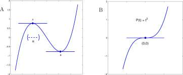
-0.5 0 0.5 1 1.5 2 2.5 -2 -1 0 1 2
Figure 3.21: A. Graph with a local maximum at A and a local minimum at B. B. Graph of P(t) = t 3 that has a horizontal tangent at (0,0); (0, 0) is neither a local maximum nor a local minimum of P.
Barn
60 ft
W
Figure 3.22: Diagram of a barn with adjacent pen bounded by a fence of length 100 feet.
Because 2W + L = 100,
L — 100 – 2W
and
A = LW = (100-2W) W
or
A = 100W – 2W 2
The question becomes now, for what value of W will A be the largest. The graph of A vs W is a parabola with its highest point at the vertex. The tangent to the parabola at the vertex is
CHAPTER 3. THE DERIVATIVE
157
horizontal, and we find a value of W for which A'(W) = 0.
(3.33)
The optimum dimensions, and L, are found by setting = 0, so that
A'(W) = 100-4^ = 0 W = 25
L = 100-2^ = 50 Thus the farmer should build a 25 by 50 foot pen.
Example 3.5.6 This problem is written on the assumption, to our knowledge untested, that spider webs have an optimum size. Seldom are they so small as 1 cm in diameter and seldom are they so large as 2 m in diameter. If they are one cm in diameter, there is a low probability of catching a flying insect; if they are 2 m in diameter they require extra strength to withstand wind and rain. We will examine circular webs, for convenience, and determine the optimum diameter for a web so that it will catch enough insects and not fall down.
Solution. Assume a circular spider web of diameter, d. It is reasonable to assume that the amount of food gathered by the web is proportional to the area, A, of the web. Because A = ird 2 /4, the amount of food gather is proportional to d 2 . We also assume that the energy required to build and maintain a web of area A is proportional to d 3 . (The basic assumption is that the work to build a square centimeter of web increases as the total web area increases because of the need to have stronger fibers. If, for example, the area of the fiber cross-section increases linearly with A and the mesh of the web is constant, the mass of the web increases as d 3 .)
With these assumptions, the net energy, E, available to the spider is of the form
E = Energy from insects caught — Energy expended building the web = k ± d 2 – k 2 d 3
where d is measured in centimeters and k\ and ki are proportionality constants.
For illustration we will assume that k\ = 0.01 and ki = 0.0001. A graph of E(d) = O.Olrf 2 — O.OOOlci 3 is shown in Figure 3.23 where it can be seen that there are two points, A and B, at which the graph has horizontal tangents. We find where the derivative is zero to locate A and B.
E'(d) = [0.0Li 2 – 0.0001d 3 ]’
= [O.OLi 2 ]’- [O.OOOld 3 ]’
= 0.01 [d 2 ]’- 0.0001 [d 3 ]’
= 0.01 x 2d- 0.0001 x 3d 2 (iv)
= 0.02d – 0.0003rf 2
(0 («)
(Hi)
(3.34)
CHAPTER 3. THE DERIVATIVE
158
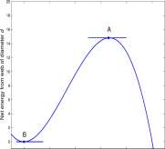
0 20 40 60 80 100
Diameter of spider web, d, in cm.
Figure 3.23: Graph of E(d) = 0.01c? 2 — O.OOOld 3 representative of the energy gain from a spider web of diameter d cm. There is a local maximum at A and a local minimum at B.
Then E'(d) = 0 yields
0.02d – 0.0003d 2 = 0 d (0.02 – 0.0003d) = 0
d = 0 or d = 0.02/0.0003 = 66.7 cm
The value d = 0 locates the local minimum at B and has an obvious interpretation: if there is no web there is no energy gain. At d — 66.7 cm, E(d) = 14.8 (units unspecified) suggests that a positive net energy will accrue with a web of diameter 66.7 cm and that weaving a web of 66.7cm diameter is the optimum strategy for the spider. Note that if our model and its parameters are correct we have determined in a rather short time what it took spiders many generations to work out. At the very least we could have moved the spiders ahead several generations with our model.
Exercises for Section 3.5, Derivatives of Polynomials, Sum and Constant Factor Rules. Exercise 3.5.1 Use Definition of the Derivative 3.22 to compute P'(t) for
Exercise 3.5.2 Suppose u and v are functions with a common domain and P = u — v. Write P(t) = u(t) + (—1) v(t) and use the Sum and Constant Factor rules to show that P'(t) = u ‘(t)-v'(t).
CHAPTER 3. THE DERIVATIVE
159
Exercise 3.5.3 Provide reasons for the steps (i) — (v) in Equations 3.32 use to show that the derivatives of quadratic functions are linear functions.
Exercise 3.5.4 a. Prove Equation 3.27, [ C ]’ = 0.
b. Prove Equation 3.28, [ t ]’ = 1.
c. Prove Equation 3.31, [ C F(t) ]’= C [ F(t) ]’.
Exercise 3.5.5 Suppose m is a positive integer and u(t) = t~ m = l/t m for t ^ 0. Show that = — mt^ m ~ 1 , thus proving the t n rule for negative integers. Begin your argument with
1 1
U lt) = hm V— L —
W b^t b-t
t m_ b m j
Exercise 3.5.6 Provide reasons for the steps (i) — (iv) in Equations 3.33 used to find the optimum dimensions of a lot adjacent to a barn.
Exercise 3.5.7 A farmer’s barn is 60 feet long on one side. He has 120 feet of fence and wishes to build a rectangular pen along that side of his barn. What should be the dimensions of the pen to maximize the the area of the pen?
Exercise 3.5.8 A farmer’s barn is 60 feet long on one side. He has 150 feet of fence and wishes to build two adjacent rectangular pens of equal area along that side of his barn. What should be the arrangement and dimensions of the pen to maximize the sum of the areas of the two pens?
Exercise 3.5.9 A farmer’s barn is 60 feet long on one side. He has 150 feet of fence and wishes to build two adjacent rectangular pens of equal area along that side of his barn. What should be the arrangement and dimensions of the pen to maximize the sum of the areas of the two pens?
Exercise 3.5.10 A farmer’s barn is 60 feet long on one side. He has 280 feet of fence and wishes to build two adjacent rectangular pens of equal area along that side of his barn. What should be the arrangement and dimensions of the pen to maximize the sum of the areas of the two pens?
Exercise 3.5.11 A farmer’s barn is 60 feet long on one side. He wishes to build a rectangular pen of area 800 square feet along that side of his barn. What should be the dimension of the pen to minimize the amount of fence used?
Exercise 3.5.12 Show that the derivatives of cubic functions are quadratic functions.
Exercise 3.5.13 Probably baseball statistics should be discussed in British units rather than metric units. Professional pitchers throw fast balls in the range of 90+ miles per hour. Suppose the pop fly ball leaves the bat traveling 60 miles per hour (88 feet/sec), in which case the height of the ball in feet will be s(t) = — 16t 2 + 88t feet above the bat, t seconds after the batter hits the ball. How high will the ball go, and how long will the catcher have to position to catch it? How fast is the ball falling when the catcher catches it?
CHAPTER 3. THE DERIVATIVE
160
Exercise 3.5.14 A squirrel falls from a tree from a height of 10 meters above the ground. At time t seconds after it slips from the tree, the squirrel is a distance s(t) = 10 — 4.9t 2 meters above the ground. How fast is the squirrel falling when it hits the ground?
Exercise 3.5.15 What is the optimum radius of the trachea when coughing? The objective is for the flow of air to create a strong force outward in the throat to clear it. For this problem you should perform the following experiment.
Hold your hand about 10 cm from your mouth and blow on it (a) with your lips compressed almost closed but with a small stream of air escaping, (b) with your mouth wide open, and (c) with your lips adjusted to create the largest force on your hand. With (a) your lips almost closed there is a high pressure causing rapid air flow but a small stream of air and little force. With (b) your mouth wide open there is a large stream of air but with little pressure so that air flow is slow. The largest force (c) is created with an intermediate opening of your lips where there is a notable pressure and rapid flow of substantial volume of air.
Let R be the normal radius of the trachea and r < R be the tracheal radius when coughing. Assume that the velocity of air flow through the trachea is proportional to pressure difference across the trachea and that the pressure difference is proportional to R — r, the constriction of the trachea. Assume that the mass of air flow is proportional to the area of the trachea (nr 2 ). Finally, the momentum, M, of the air flow is mass times velocity:
What value of r, 0 < r < R, maximizes Ml
Exercise 3.5.16 Cite formulas that justify the steps (i) — (iv) in Equations 3.34 for the analysis of the spider web.
Exercise 3.5.17 Let P(t) = — 3 + 5t — 2t 2 . Cite the formulas that justify steps (i) — (vi) below:
M = kr 2 (R-r)
P’
(t)
[-3 + 5 t + (-2) t 2 ]’
[-3]’ + [5 t}’ + [(-2) t 2 ]’
(ii
0 + [5 x + [(-2) t 2 }’
(Hi
0 + 5 [t]’ + (
2) [t 2 ]’
iv
0 + 5 x1 + (
2) [t 2 ]’
(v
0 + 5 x1 + (
2) x 2t
(vi
= 5-4*
Exercise 3.5.18 Compute the derivatives of the following polynomials as in the previous exercises.
CHAPTER 3. THE DERIVATIVE
161
Use only one rule for each step written, and write the name of the rule used for each step.
a. P(t) = 15t 2 – 32t 6 c. P(t) = T + f
b. P(t) = l+t + t 2 + t 3 d. P(t) = (1 + t 2 ) 2 e. Pit) = 31t 52 – 82t 241 + vrf 314 f. Pit) = 2 5 + 17t 5
g. Pit) = V2-4r7 + 18t 35 h. Pit) = 17 3 -Ln + 5t 705
Exercise 3.5.19 Find values of t for which P\t) = 0 for:
Exercise 3.5.20 Suppose that in the problem of Example 3.5.6, the work of building a web is proportional to <i 4 , the fourth power of the diameter, d. Then the energy available to the spider is
E = hd 2 -k 2 d 4
Assume that h = 0.01 and k 2 = 0.000001.
a. Draw a graph of E = 0.01 d 2 – 0.000001 d A for -10 < d < 110.
b. Find E\d) for E(d) = 0.01 d 2 – 0.000001 d 4 .
c. Find two numbers, d, for which E’id) = 0.
d. Find the highest point of the graph between d = 0 and d = 100.
Exercise 3.5.21 Consider a territorial bird that harvests only in its defended territory (assumed to be circular in shape). The amount of food available can be assumed to be proportional to the area of the territory and therefore proportional to d 2 , the square of the diameter of the territory. Assume that the food gathered is proportional to the amount of food available times the time spent gathering food. Let the unit of time be one day, and suppose the amount of time spent defending the territory is proportional to the length of the territory boundary and therefore equal to k x d for some constant, k. Then 1 — kd is the amount of time available to gather food, and the amount, F of food gathered will be