
part0004
- Page ID
- 24590
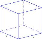
0 < x < ^ insures that no side of the box is a negative number. A graph of V appears in
Figure 8.6B. The dashed line shows an extension of the graph of y = (4 — 2x)(3 — 2x)x that is not
part of the graph of V. Compute V’:
V = [(4 – 2z)(3 – 2x)x]’
= [(4 – 2x)]’ (3 – 2x)x + (4 – 2x) [(3 – 2x)x]’
= [(4 – 2x))’ (3 – 2x)x + (4 – 2x) [(3 – 2x)]’ x + (4 – 2x) (3 – 2x) [a;]’
V = 8x 2 – 28a;+ 12 Find the critical points:
• V = 0
V 1 = 0 implies 8a; 2 — 28a; + 12 = 0 implies x = 3 or x = –
x = j is in the domain of V but x = 3 is not.
• V does not exist. No such points. V is a cubic function and has derivatives at every point.
Q
• End points. The end points are x = 0 and x = ^
The three critical values of x are 0, | and | Find the maximum V:
3 2
The maximum volume is 3 and occurs with a;
CHAPTER 8. APPLICATIONS OF DERIVATIVES
354
In the preceding Example, we were given a surface area and asked to find the dimensions that will maximize the volume. A dual problem is to be given a required volume, find the dimensions that will minimize the required surface
Example 8.2.2 Suppose a box with a square base and closed top and bottom is to have a volume of 8 cubic meters. What dimensions of the box will minimize the surface area of the box?
Solution. Let x be the length of one side of the square base and y be the height of the box. Then the volume and surface area of the box are
V = x 2 y S = 2x 2 + 4xy
Because V is specified to be 8 cubic meters
8 = x 2 y so that We substitute for y in the expression for S and get
y = s
X
X
^ „ o 8 „ n 32 S = 2x 2 + Ax^ = 2x 2 + —
X X
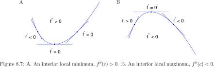
Figure for Example 8.2.2.2 A. Box with square bottom and volume = 8 m 3 . B. Graph of the
function, S(x) = 2x 2 +
32
A
B
V = 2 x” + 32/x
Length of side, x
The domain of S is x > 0 (there are no endpoints, x = 0 is not allowed by the x in the denominator and there is no upper limit on x). Then
S'{x)
32
x
2x 2
[2x 2 ]’ + [32a;1
= 4x-32x~ 2
S'(x) exists for all x > 0 and S'(x) = 0 yields
4x – 32x~ 2 = 0, 4x 3 – 32 = 0, x = 2 m
Thus we conclude that the base of the box should be 2 by 2 and because x 2 y = 8 the height y of the box should also be 2. Examination of the graph of S(x) = 2x 2 + ^ in Example Figure 8.2.2.2B suggests it is a minimum (and not, for example, a maximum!).
CHAPTER 8. APPLICATIONS OF DERIVATIVES
355
8.2.1 The Second Derivative Test.
There is a clever way of distinguishing local maxima from local minima using the second derivative. The following theorem is proved in Section 12.2.
Theorem 12.2.3. Suppose / is a function with continuous first and second derivatives throughout an interval [a, b] and c is a number between a and b for which f'(c) = 0. Under these conditions:
1. If f”{c) > 0 then c is a local minimum for / (see Figure 8.7A).
2. If f”(c) < 0 then c is a local maximum for / (see Figure 8.7B).
In Example 8.2.2, S'(x) = 4(x – 8x 2 ), so that
S”{x)
4 x
57′
-2
4 1 + 16x
-3
Now S'(2) = 0, and S”(2) = 12 > 0, so by the second derivative test, x = 2 is a local minimum for S, as we previously concluded.
Example 8.2.3 The salmon and tuna cans shown in Example Figure 8.2.3.3 both contain fish. Why are they shaped so differently?
Suppose the criterion for making cans is to minimize the amount of metal required to hold a fixed amount of fish (the cans show Net Wt. 14.5 oz and 16 oz; we did not find cans holding equal weights of fish). Which can most closely meets the criterion?
Figure for Example 8.2.3.3 A. Salmon and tuna cans.

CHAPTER 8. APPLICATIONS OF DERIVATIVES
356
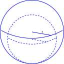
Question: Of all cans of volume equal to 1, which has the smallest surface area?
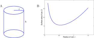
Assume that the ‘can’ (cylinder) in Example Figure 8.2.3.3 has volume equal to 1. The area of the top end of the can is nr 2 and the circumference of the top lid is 2irr. The volume, V, of the can is
V = nr 2 h
and the surface area, S, of the can is
S = 2ixr 2 + 2ttt h
Figure for Example 8.2.3.3 A. A can of volume 1. B. A graph of S(r) = 2irr 2 + £
The requirement that the volume be 1 yields
1 = wr 2 h and solving for h yields h = — 5 We substitute this value into the expression for S and obtain
S = 2rrr 2 + 2tit
1
S = 2nr z
TIT
The domain for S is r > 0 (there are no endpoints).
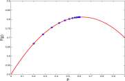
From the graph of S in Figure 8.2.3.3B it appears that there is a single minimum at about r = 0.5. We find the critical points.
S\t)
The requirement S'(r) = 0 yields 4?rr — 2r~ 1
Aixr – 2r 2
‘2n
0.542
Recall that h = so that the ratio of h to r (height to radius ratio) that gives minimum surface area is
h 1/nr 2
r
r
r=l/V2^
TIT
r=l/\/2n
Thus the height should be twice the radius, or equal to the diameter.
CHAPTER 8. APPLICATIONS OF DERIVATIVES
357
8.2.2 How to solve these problems.
There are some procedures we have been using that will help you solve these problems. They are listed in rough order of use and applied to an example.
• Read the problem!
Problem: Find the rectangle of largest area that can be inscribed in a semicircle of radius 1.
• Draw a picture. (Representative of the problem!)
Picture should have a semicircle of radius 1 and a rectangle inscribed in it. Also draw a radius to a corner of the rectangle. Figure 8.8A.
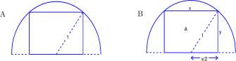
Figure 8.8: A. A semicircle of radius 1 with inscribed rectangle. B. Labels for the diagram in A.
• Label parts of the picture. This will introduce symbols for important parameters of the problem.
x and y should label horizontal and vertical sides of the rectangle, and A is the area of the rectangle. Figure 8.8B.
• Write relations between the parameters.
(f ) 2 + y 2 = 1 an d a = % y-
• Write a function of a single variable. Write the parameter to be optimized in terms of a single adjustable parameter (variable).
Solve for y in f |) + y 2 = 1 and substitute into A = xy.
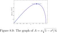
A = xJl – x 2 /A
• Draw a graph. It is usually easy to draw a graph of your function on a calculator and the graph will often reveal the maximum and minimum points. You may end the process at this step with a calculator based estimate of the answer. A graph of A = xJl — a; 2 /4 appears in Figure 8.9 and the maximum appears to be about x = 1.5.
• Look for a clever simplification.
The value of x that minimizes A also minimizes A 2 and A 2 = x 2 — x A /4. You have your choice: Compute the derivative of A = xJl — x 2 /4 or compute the derivative of A 2 = x 2 -x 4 /4. (Choose A 2 !!)
CHAPTER 8. APPLICATIONS OF DERIVATIVES
358
Find the critical points. Compute the first derivative; find where it is zero or fails to exist; examine the end points.
A 2
A
2x — x 3 exists for all x
x = 0 or x — \[2
The critical points are x = \[2 and the end points x = 0 and x — 2.
A 2 (0) = 0, A 2 (y/2) = 1, A 2 (2) = 0. At this stage we know that x = y/2 maximizes A 2 (x) because the maximum has to occur at one of the critical points. For illustrations, we also:
Use the second derivative test, if needed and applicable.
A
2-3x 2
A’
–V2
[A 2
–V2
IS
negative, so x = \[2 is a local maximum. To see that it is actually a maximum,
we have to check the other critical points.
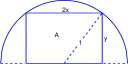
Explore 8.2.1 Selection of labels on a figure can simplify or complicate the equations you derive. The previous figure is shown with the horizontal side of the rectangle being 2x instead of x. Write
Yy 1
the equations that correspond to . , analysis.
1, A = xy and A = xJl — x 2 /A from the previous
Figure for Exercise 8.2.0 Improved labels for Figure 8.8A.
Example 8.2.4 Snell’s Law When you see a fish in a lake it typically is below where it appears to be. A spear, arrow, bullet, rock or other projectile launched toward the image of the fish that you see will pass above the fish. The different speeds of light in air and in water cause the light beam traveling from the fish to your eye to bend at the surface of the lake. The apparent location of the fish is marked as a dotted fish in Figure 8.2.4.4.
CHAPTER 8. APPLICATIONS OF DERIVATIVES
359
Figure for Example 8.2.4.4 A. Light ray from fish to observer. The dotted fish is the apparent
location of the fish.
O,
Apparent
Pierre Fermat asserted in 1662 that the path of the light beam will be that path that minimizes the total time of travel in the two media. The speed of light in water, v%, is about 0.75 times the speed of light in air, v\. Suppose d is the horizontal distance between your eye and the fish, hi is the height of your eye above the water and h 2 is the depth of the fish below the surface of the lake. Finally let x be the horizontal distance between your eye and the point at which the beam passes through the surface of the lake.
Figure for Example 8.2.4.4 B. Light ray from fish to observer with labels.

I-
9 A
-I
The distances the light ray travels in air and water are
Air distance: \jh\-\- x 2 Water distance: \jh\ + (d — x) 2 The times that the light spends traversing air and traversing water are (distance/velocity)
Air time:
h 2 + x 2
Water time:
y/h 2 2 + (d- Xf
Vl v 2 The total time, T, for the ray to travel from the fish to your eye is
Jh 2 + x 2 Jh 2 + (d-x) 2 T=^ + -*—= 0<x<d
“i
CHAPTER 8. APPLICATIONS OF DERIVATIVES
360
Our task is to find the value of x that minimizes T. A graph of T is shown for values V\ — 1, v 2 = 0.75, d = 10 meters, hi — 2 meters, /12 = 3 meters. As tempting as it may be, it is not the time to get clever and square each term in the previous equation, for it is not generally true that
(a + bf
+ b 2 . Instead we compute T’ directly and find that
x
d
X
r
h% + {d
X)
V2
Figure for Example 8.2.4.4 Transit time for a light ray from fish to observer for parameter values v\ = 1, v 2 = 0.75, d — 10 meters, hi = 2 meters, h 2 = 3 meters. The distance, x, for which the transit time is minimum is a bit less that 7 meters. v a is the velocity of light in air.
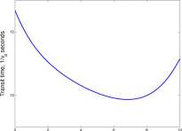
Distance, meters
Setting T’ = 0 and solving for x is not advised. We take a qualitative approach instead, and return to the geometry and identify two angles, Q\ and 6? 2 , the angles the light ray makes with a vertical line through the point of intersection with the surface. They are marked in both figures 8.2.4.4 and 8.2.4.4. It may be seen that
x
hi
sin 81
and
d
x
x c
y/h 2 2 + (d-x)<
sin do
and
T’
sin 81 sin 8 2
Vi v 2
Observe from the geometry that as x moves from 0 to d, 8\ increases from 0 to a positive number and 8 2 decreases from a positive number to 0. There is a single value of x where the graphs of
sinfj*!
Vl
and
sin do
Vo
cross and at that point T’ = 0 and
sin 81 sin 8 2
Vl v 2
Equation 8.4 is referred to as Snell’s law and applies to many problems of optics. Because for water and air, v 2 = 0.75 V\, and we would have
(8.4)
sin 8\ sin 8 2 vi 0.75fi
or
sin 81
~1T
sin 8 2 0.75
CHAPTER 8. APPLICATIONS OF DERIVATIVES
361
we would have
sin 6\ > sin 9 2 or 9i > 9 2
which implies that the light ray bends down into the water as shown, and the fish is actually below its apparent position.
Exercises for Section 8.2, Some Traditional Max-Min Problems.
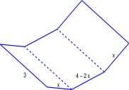
Exercise 8.2.1 Suppose you have a 3 meter by 4 meter sheet of tin and you wish to make a box that has tin on the bottom and on two opposite sides. The other two sides are of wood that is in plentiful supply. You are going to make a rectangular box by folding up panels of width x across the ends that are 3 meters wide as shown in Figure 8.2.1. What value of x will maximize the volume of the box and what is the volume?
Figure for Exercise 8.2.1 Diagram for Exercise 8.2.1.
Exercise 8.2.2 In Exercise 8.2.1, would it be better (make a box of larger volume) to fold up panels of width x across the sides that are 4 meters long?
Exercise 8.2.3 Dissatisfied with having to discard the four corners as in Example 8.2.1, you decide to take another approach. From the 3 by 4 meter panel, you will cut two strips of width x across an end that is 3 meters wide, fold up two similar strips of width x and use the first two strips to make the other sides. See Figure 8.2.3. The two strips you cut may be too long, so that you may still have to discard some tin. What value of x will make a box of the largest volume and what is the volume?
Figure for Exercise 8.2.3 Diagram for Exercise 8.2.3.
XXX X
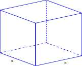
Exercise 8.2.4 A box with a square base and open top has surface area of 12 square meters (Figure 8.2.4. What dimensions of the box will maximize the volume?
Figure for Exercise 8.2.4 Box with square base and surface area = 12 m 2 4 for Exercise 8.2.4.
y
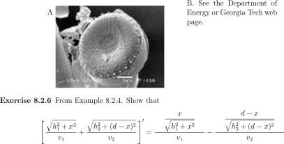
Exercise 8.2.5 Electron micrographs of diatoms are shown in Exercise Figure 8.2.5. Diatoms are phytoplankton that originated some 200 million years ago and are found in marine, fresh water and moist terrestrial environments, and contribute some 45 percent of the oceans organic production. The shells of the diatoms illustrated are like pill boxes (a cylindrical cup caps another cylindrical cup and a ‘girdle’ surrounds the overlap of the shells) and some parts are permeable and other parts appear to be impermeable. (Other diatoms have quite different structures, oblong and pennate, for example.) Typically the structure of such shells optimize some aspect of the organism, subject to functional constraints. Make measurements of the diatoms and discuss the optimality of the use of materials to make the shell, with the constraint that light must penetrate the shell.
Figure for Exercise 8.2.5 Electron micrographs of diatoms for Exercise 8.2.5. A. Cyclotella comta is the dominant component of the spring diatom bloom in Lake Superior, http://www.glerl.noaa.gov/seagrant/G...s/Diatoms.html B. Thalassiosira pseudonana, the first eukaryotic marine phytoplankton for which the whole genome was sequenced. Micrograph by Nils Kroger, Universitat Regensburg, from http://www.jgi.doe.gov/News/news_9_30_04.html or from http://gtresearchnews.gatech.edu/new...-structure.htm
CHAPTER 8. APPLICATIONS OF DERIVATIVES
363
Exercise 8.2.7 Find the area of the largest rectangle that can be inscribed in a right triangle with sides of length 3 and 4 and hypotenuse of length 5.
Exercise 8.2.8 Two rectangular pens of equal circci Eire to be made with 120 meters of fence. An exterior fence surrounding a rectangle is first constructed and then an interior fence that partitions the rectangle into two equal areas is constructed. What dimensions of the pens will maximize the total area of the two pens?
Exercise 8.2.9 A dog kennel with four pens each of area 7 square meters is to be constructed. An exterior fence surrounding a rectangular area is to be built of fence costing $20 per meter. That rectangular area is then to be partitioned by three fences that are all parallel to a single side of the original rectangle and using fence that costs $10 per meter. What dimensions of pens will minimize the cost of fence used?
Exercise 8.2.10 A ladder is to be put against a wall that has a 2 meter tall fence that is 1 meter away from the wall. What is the shortest ladder that will reach from the ground to the wall and go above the fence?
Exercise 8.2.11 a. What is the length of the longest ladder than can be carried horizontally along a 2 meter wide hallway and turned a corner into a 1 meter hallway? Suppose the floor to ceiling height in both hallways is 3 meters, b. What is the longest pipe that can be carried around the corner?
Exercise 8.2.12 A box with a square base and with a top and bottom and a shelf entirely across the interior is to be made. The total surface area of all material is to be 9 m 2 . What dimensions of the box will maximize the volume?
Exercise 8.2.13 A rectangular box with square base and with top and bottom and a shelf entirely across the interior is to have 12 m 3 volume. What dimensions of the box will minimize the material used?
Exercise 8.2.14 A box with no top is to be made from a 22 cm by 28 cm piece of card board by cutting squares of equal size from each corner and folding up the ‘tabs’. What size of squares should be cut from each corner to make the box of largest volume?
Exercise 8.2.15 A shelter is to be made with a 3 meter by 4 meter canvas sheet. There are equally spaced grommets at one meter intervals along the 4-meter edges of the canvas. Ropes are tied to the four grommets that are one meter from a corner and stretched, so that there is a two-meter by three-meter horizontal sheet with two one-meter by three-meter flaps on two sides. The other two sides are open. The two flaps are to be staked at the corners so that the flaps slope away from the region below the horizontal portion of the canvas. How high should the horizontal section be in order to maximize the volume of the shelter?
Exercise 8.2.16 An orange juice can has volume of 48-7T cm 3 and has metal ends and cardboard sides. The metal costs 3 times as much as the card board. What dimensions of the can will minimize the cost of material?
Exercise 8.2.17 The ‘strength’ of a rectangular wood beam with one side vertical is proportional to its width and the square of its depth. A sawyer is to cut a single beam from a 1 meter diameter log. What dimensions should he cut the beam in order to maximize the strength of the beam?
CHAPTER 8. APPLICATIONS OF DERIVATIVES
364
Exercise 8.2.18 A rectangular wood beam with one side vertical has a ‘stiffness’ that is proportional to its width and the cube of its depth. A sawyer is to cut a single beam from a 1 meter diameter log. What dimensions should he cut the beam in order to maximize the stiffness of the beam?
Exercise 8.2.19 A life guard at a sea shore sees a swimmer in distress 70 meters down the beach and 30 meters from shore. She can run 4 meters/sec and swim 1 meter per second. What path should she follow in order to reach the swimmer in minimum time?
Exercise 8.2.20 You stand on a bluff above a quiet lake and observe the reflection of a mountain top in the lake. Light from the mountain top strikes the lake and is reflected back to your eye, the path followed, by Fermat’s hypothesis, being that path that takes the least time. Show that the angle of incidence is equal to the angle of reflection. That is, show that the angle the beam from the mountain top to the point of reflection on the lake makes with the horizontal surface of the lake (the angle of incidence) is equal to the angle the beam from the point of reflection to your eye makes with the horizontal surface of the lake (the angle of reflection). Let v a denote the velocity of light in air.
Exercise 8.2.21 Two light bulbs of different intensities are a distance, d, apart. At any point, the light intensity from one of the bulbs is proportional to the intensity of the bulb and inversely proportional to the square of the distance from the bulb. Find the point between the two bulbs at which the sum of the intensities of light from the two bulbs is minimum.
Exercise 8.2.22 An equation for continuous logistics population growth is
where P is population size, R is the low density growth rate, and M is the carrying capacity of the environment. For what value of P will the growth rate, P’ be the greatest?
Exercise 8.2.23 Ricker’s model for population growth is
where P is population size, R is the low density growth rate, and a reflects the carrying capacity of the environment. For what value of P will the growth rate, P’ be greatest?
Exercise 8.2.24 A comet follows the parabolic path, y = x 2 and Earth is at (3,8). How close does the comet come to Earth?
Exercise 8.2.25 A tepee is to be covered with 30 buffalo skins. What should be the angle at the base of the tepee that will maximize the volume inside the tepee?
Note: The volume of a right circular cone with base radius r and height h is irr 2 h/3 and its lateral surface area is nr^/r 2 + h 2 .
Exercise 8.2.26 A very challenging exercise. A tepee is to be covered with 30 buffalo skins. The skins are a little longer than the height of the Indians that will be inside and not quite as wide as the height of the Indians. Thus the areas of the skins are approximately the square of the height of the Indians. The Indians wish to maximize the area inside the teepee in which they can walk standing upright. What angle at the base of the teepee will maximize that area?

P’ =
p
RPe~
CHAPTER 8. APPLICATIONS OF DERIVATIVES
365
8.3 Life Sciences Optima
Natural selection constantly optimizes life forms for reproductive success. Consequently, optima are endemic in living organisms and groups of organisms, but they are typically difficult to describe and analyze and vary with the organism. Biology optima are never as simple as the geometry problems of the previous sections, such as, “What is the size of the largest cube that can fit in a sphere?” An otherwise square cell confined to live in a sphere is very likely to become a sphere. Typically the optimum is a balance between opposing requirements as in the simplified model 1 of cell size included here. A few such problems are supplied for your analysis.
Example 8.3.1 Mathematical Model 8.3.1 Consider a bacterium that grows as a sphere, such as streptococcus. Its reproductive success is proportional to the energy that it produces.
1. Energy production is proportional to cell volume which provides space for processing and storage of nutrients.
2. Energy production is proportional to the concentration of nutrients inside the cell, which in turn is proportional to the ratio of the surface area of the cell to the volume of the cell.
If we concentrate only on component 1, we might write
Energy Production = A V
where A is a positive constant. Energy Productioni will be large if V is large and streptococcus cell size should increase without bound.
If we concentrate only on component 2, we might write
S 1 Energy Production 2 = B 0 — = B
v yv
where B is a positive constant (for streptococcus cells which grow in the shape of a sphere,
S = v^36~7r V 2 / 3 ). Energy Production will be large if V is small and streptococcus cell size should
decrease – to zero with no nutrient processing organs!
Large cells have large capacity for energy production, but are inefficient because of low nutrient concentration. Small cells have high nutrient concentration, but may have limited capacity to use the nutrients.
Caution: Smoke and mirrors ahead. How do we combine the two expressions of Energy Production? We choose the harmonic mean of the two. The harmonic mean of n numbers {ax, a 2 , • • •, a n } is defined by
n
Harmonic mean = -j j j- (8.5)
Explore 8.3.1 The harmonic mean is useful for combining rates. Suppose you travel from city A to city B at rate r mph and travel from B back to A at a rate s mph. Show that the rate of the round trip is the harmonic mean of r and s.
1 A much more satisfactory model and analysis is presented in Kohei Yoshiyama and Christopher A. Klausmeier, Optimal cell size for resource uptake in fluids: A new facet of resource competition. American Naturalist 171 (2008), pp. 59-79
CHAPTER 8. APPLICATIONS OF DERIVATIVES
366
Now lets write the harmonic mean of the two Energy Productions as
Energy Production
1/3
+
AV B/V 1 / 3
2A V B/V AV + B/V 1/3
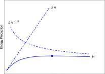
For illustration purposes, suppose A = B = 1 and examine the function
H(V)
2V V~ l,z
v + v1/3 ‘
Shown in Figure 8.3.1.1 are the graphs of y = 2V, y = 2V~ 1/3 and H. When V < 1, V~ 1/3 > V and the denominator is ~ V^ 1 ^ 3 and cancels the factor V~ x l 3 in the numerator. Consequently, when 7< 1, H(V) ~ 2V and close to zero. Similarly, when V 3> 1, H(V) ~ V^ 1 ^ 3 and is close to zero. There is an intermediate value of V for which H is maximum. You are asked to find that value in Exercise 8.3.1.
We have shown that the competing requirements of large capacity and high nutrient concentrations can be balanced to achieve an intermediate optimum cell size. We are ignorant of the values of A and B and have selected the harmonic mean only as a reasonably unbiased means of combining the two functions.
Figure for Example 8.3.1.1 Graphs of y = 2V, y = 2V^ 3 and H(V) = 2V V^/iV + V’ 1 /’ 3 ).
Cell Volume
Exercises for Section 8.3, Life Sciences Optima
Exercise 8.3.1 Find the maximum value of H(V) = 2V V~ l/3 /(V + V~ 1/3 ) for V > 0.
Exercise 8.3.2 The island body size rule states that when an ecosystem becomes isolated on an island, say by rising sea levels, the species of large body size tend to evolve to a smaller body size, and species of small body size tend to increase in size. Craig McClain et al 2 found a similar contrast in the sea between shallow water where nutrient levels are high and deep water (depth greater than 200 meters) where nutrient levels are low. Gastropod genera that have large
2 Craig R. McClain, Alison G. Boyer and Gary Rosenberg, The island rule and the evolution of body size in the deep sea, Journal of Biogeography 33 (2008), pp 1578-1584.
CHAPTER 8. APPLICATIONS OF DERIVATIVES
367
shallow-water species tend to have smaller deep-water representatives; those that have small shallow water species tend to have larger deep-water species.
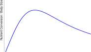
Suppose the ratio of nutrient conversion to body size vs body size is similar to the graph in Figure 8.3.2 and that at high nutrient concentrations, nutrient conversion is not the limiting factor
– predation and mate finding, for example, may be more important. Suppose further that a low nutrient concentrations, nutrient conversion becomes more important and nutrient conversion/body size must be greater than that for high nutrient levels. How is the graph consistent with the observed differences in body size?
Figure for Exercise 8.3.2 Hypothetical graph of the ratio of nutrient production to gastropod
body size vs body size.
Exercise 8.3.3 Some small song birds intermittently flap their wings and glide with wings folded between flapping sessions. Why? R. M. Alexander 3 suggests the following analysis. The power required to propel an airplane at a speed u is
where A and B are constants specific to the airplane and L is the upward force that lifts the plane. Au 3 represents the drag on the airplane due largely to the air striking the front of the craft.
a. For what speed is the required power the smallest?
b. The energy required to propel the airplane is E = P/u. For what speed is the energy required to propel the plane the smallest.
c. How does the speed of minimum energy compare with the speed of minimum power?
d. Suppose a bird has drag coefficient A b with wings folded and A b + A w with wings extended and flapping, and let x be the fraction of time the bird spends flapping its wings. Suppose that the speed of the bird while flapping its wings is the same as the speed when the wings are folded and that all of the lift is provided when the wings are flapping. The lift over one complete cycle should be
3 R. McNeill Alexander, “Optima for Animals” Princeton University Press, Princeton, NJ, 1996, Section 3.1, pp
Gastropod Size
P = Au 3 + BL 2 /u

CHAPTER 8. APPLICATIONS OF DERIVATIVES
368
where m is the mass of the bird. Then the power required while flapping is
^flapping = (A b + A w )u 3 + B
(
rag
)
2 1
x
u
Write an expression for Pfoided-
c. The average power over a whole cycle should be
P = (1 – x)P fo i dcd + a;P fl .
= A b u 3 + xA w u 3 + B
2 2
m g
apping
XU
Find the value of x for which the average power over the whole cycle is minimum.
f. The average energy over a whole cycle is E = P/u. For what value of x is the average energy a minimum?
This problem is continued in Exercise 13.2.12
Alexander further notes that it may be necessary to consider also the efficiency of muscle contraction at different flapping rates.
Exercise 8.3.4 Read the amazing story of the kakapo at
http://evolution.berkeley.edu/evolib.../060401_kakapo and the Wikipedia entry on kakapo. You might assume that in really good times, only males would be born and in really bad times only females would be born. Why is it that both males and females are retained in the natural population?
The next three exercises could form the basis of a semester project.
Exercise 8.3.5 Sickle cell anemia is an inherited blood disease in which the body makes sickle-shaped red blood cells. It is caused by a single mutation from glutamic acid to valine at position 6 in the protein Hemoglobin B. The gene for hemoglobin B is on human chromosome 11; a single nucleotide change in the codon for the glutamic acid, GAG, to GTG causes the change from glutamic acid to valine. The location of a genetic variation is called a locus and the different genetic values (GAG and GTG) at the location are called alleles.
People who have GAG on one copy of chromosome 11 and GTG on the other copy are said to be heterozygous and do not have sickle cell anemia and have elevated resistance to malaria over those who have GAG on both copies of chromosome 11. Those who have GTG on both copies of chromosome 11 are said to be homozygous and have sickle cell anemia – the hydrophobic valine allows aggregation of hemoglobin molecules within the blood cell causing a sickle-like deformation that does not move easily through blood vessels.
Let A denote presence of GAG and a denote presence of GTG on chromosome 11, and let AA, Aa and aa denote the various presences of those codons on the two chromosomes of a person (note: Aa = a A); AA, Aa and aa label are the genotypes of the person with respect to this locus. It is necessary to assume non-overlapping generations, meaning that all members of the population are simultaneously born, grow to sexual maturity, mate, leave offspring and die. Let P, Q and R denote the frequencies of A A, Aa and aa genotypes in a breeding population and let p and q denote the frequencies of the alleles A and a among the chromosomes in the same population. The frequencies P, Q, and R are referred to as genotype frequencies and p and q are referred to as allele frequencies. In a population of size, N, there will be 2_V chromosomes and P x 2N + Q x N of the chromosomes will be A.
CHAPTER 8. APPLICATIONS OF DERIVATIVES
369
In a mating of AA with Aa adults, the chromosome in the fertilized egg (zygote) obtained from A A must be A and the chromosome obtained from Aa will be A with probability 1/2 and will be a with probability 1/2. Therefore, the zygote will be AA with probability 1/2 and will be Aa with probability 1/2.
a. Show that the allele frequencies p and q in a breeding population with genotype frequencies P, Q and R are given by
P = P+\Q and q = + R.
b. Assume a closed population (no migration) with random mating and no selection. Complete the table showing probabilities of zygote type in the offspring for the various mating possibilities, the frequencies of the mating possibilities, and the zygote genotype frequencies. Include zeros with the zygote type probabilities but omit the zeros in the zygote genotype frequencies. Random mating assumes that the selection of mating partners is independent of the genotypes of the partners.
c. When the table is complete, you should see that
S Aa = ^PQ + PR+^QP + ^Q 2 + l -QR + RP+ l -QR
= PQ + 2PR+ l -Q 2 + QR = 2P Qq + R^j + Q Qq + R^j
= (2P + q)(±q + r) = i(p+\q) (\q + r )
= 2pq
Show that
Saa = P 2 and S aa = q 2
This means that under the random mating hypothesis, the zygote genotype frequencies of the offspring population are determined by the allele frequencies of the adults. This is referred to as the Hardy-Weinberg theorem. If the probability of an egg growing to adult and
CHAPTER 8. APPLICATIONS OF DERIVATIVES
370
contributing to the next generation of eggs is the same for all eggs, independent of genotype, then the allele frequencies, p and q, are constant after the first generation.
Random mating does not imply the promiscuity that might be imagined. It means that the selection of mating partner is independent of the genotype of the partner. In the United States, blood type would be a random mating locus; seldom does a United States young person inquire about the blood type of an attractive partner. In Japan, however, this seems to be a big deal, to the point that dating services arranging matches also match blood type. The major histocompatibility complex (MHC) of a young person would seem to be fairly neutral; few people even know their MHC type. It has been demonstrated, however, that young women are repulsed by the smell of men of the same MHC type as their own 4 .
d. Show that in a closed random mating population with no selection, if the frequency of A in the adults in one generation is p, then the frequency of A in adults in the next generation will also be p.
e. Suppose that because of malaria, an AA type egg, either male or female, has probability 0.8 of reaching maturity and mating and because of sickle cell anemia an aa type has only 0.2 probability of mating, but that an Aa type has 1.0 probability of mating. This condition is called selection. Then the distribution of genotypes in the egg and the mating populations will be
Genotype AA Aa aa Egg p 2 2pq q 2
Adult Q.8p 2 /F 2pq/F 0.2q 2 /F where F = 0.8p 2 + 2pq + 0.2q 2
Find the frequency of A in the adult population. Note: This will also be the frequency of A in the next egg population.
f. We call F{p) the balance of the population, and because p + q = 1
F = F(p) = 0.8p 2 + 2p(l -p) + 0.2(1 – pf
You will be asked in Exercise 8.3.8 to show that when the probability of reproduction depends on the genotype {selection is present), during succeeding generations, allele frequency, p, moves toward the value of local maximum of F.
1. Show that F(p) = 1 – 0.2p 2 – 0.8(1 – pf.
2. Find the value p of p that maximizes F{p).
Exercise 8.3.6 Consider two alleles A and a at a locus of a random mating population and the fractions of AA, Aa and aa zygotes that reach maturity and mate are in the ratio 1 + «i : 1 : 1 + s 2 where Si and s 2 can be positive, negative, or zero, but s± > — 1 and s 2 > — 1- The balance function is
where p and q are the frequencies of A and a among the zygotes.
4 Claus Wedekind, et al, MHC-Dependent mate preferences in humans, Proceedings: Biological Sciences, 260 (1995)
F(p) = (1 + Sl )p 2 + 2pq + (1 + s 2 )q 2
(1 + Sl )p 2 + 2p(l p ) + (l + S2 )(l – p) 2 1 + s 1 p 2 + s 2 {l-pf
245-249.
CHAPTER 8. APPLICATIONS OF DERIVATIVES
371
a. Sketch the graphs of F and find the values p of p in [0,1] for which F(p) is a maximum for
1. si = 0.2 and s 2 = -0.3.
2. si = 0 and s 2 = -0.2.
3. si = —0.2 and s 2 = —0.3.
4. si = 0.2 and s 2 = 0.3.
b. Suppose that si + s 2 ^ 0 and 0 < s 2 /(s\ + s 2 ) < 1. Is it true that ps 2 / (si + s 2 ) is the value of p in [0,1] for which -F(p) is a maximum?
Exercise 8.3.7 Use the notation of the previous exercise, Exercise 8.3.6.
a. Run the following MATLAB program.
close all;clc;clear p=0.2;q=l-p;sl=-0.3;s2=-0.5; for k = 1:12 pp(k) = p;
AA = p~2; Aa = 2*p*q; aa = q~2; F(k) = (l+sl)*AA + Aa + (l+s2)*aa; AA_n = (l+sl)*AA/F(k); Aa_n = Aa/F(k); aa_n = (l+s2)*aa/F(k); p = AA_n+0.5*Aa_n; q = 0.5*Aa_n+aa_n; end
[pp.’ F.’] x = [0:0.02:1]; y = l+sl*x.~2 +s2*(l-x).”2; plot(x,y,’r’,’linewidth’,2) xlabeK’p’ , ‘fontsize’ ,16); ylabel(‘F(p) ‘, ‘fontsize’,16) hold(‘on’)
plot(pp,F,’o’,’linewidth’,2)
b. The program computes the allele frequency, p, of allele A through 12 generations of selection and produces the graph shown to the left of the program. Mark the initial and second, third and fourth values of p. What is the limiting value of pi
c. Change the second line of the program to p=0.9; q=l-p; sl=-0.3; s2=-0.5; , and run the new program.
d. Change the second line of the program to p=0.2; q=l-p; sl=0.3; s2=0.5; , and run the new program.
e. Use some other values of p , si , and s2 , and run the program.
CHAPTER 8. APPLICATIONS OF DERIVATIVES
372
Exercise 8.3.8 The program shown in Exercise 8.3.7 assumes a population with an A-allele frequency of p=0.2 and computes future populations assuming that there is selection pattern AA: 0.7; Aa: 1.0; aa: 0.5. The heterozygote, Aa, is favored over either of the two homozygotes, AA and aa; the condition is referred to as over dominance and occurs in sickle cell anemia. The A-allele frequency of p=0.2 is out of balance with the selection forces acting on the population, and in subsequent generations p moves toward the value p that maximizes the balance function,
F(p) = (l + s 1 )p 2 + 2pq+(l + s 2 )q 2 = (1 + Sl ) p 2 + 2p (1 – p) + (1 + s 2 ) (1 – pf
= l + s lP 2 + s 2 {l-p) 2 .
This exercise proves that it always happens in the case of over dominance.
a. Consider two alleles A and a at a locus of a random mating population with non-overlapping generations and the fractions of AA, Aa and aa zygotes that reach maturity and mate are in the ratio 1 + s± : 1 : 1 + s 2 where — 1 < s 1 < 0 and — 1 < s 2 < 0. Show that the maximum value of
F(p) = 1 + si p + s 2 (1 — p) occurs at p = and Fip) = 1 H < 1.
Sl + S 2 ‘ Si + s 2
b. Assume the egg allele frequencies in the first generation are A p 0 and a go = 1 — Po and that the egg genotype frequencies are AA pi, Aa 2p 0 q 0 and aa q 2 . After selection the adult genotype frequencies are
AA Aa aa
(1 + Si)Pq 2p 0 q 0 (1 + s 2 )ql where F(p 0 ) = 1 + Si p\ + s 2 (1 – p 0 ) 2 F(po) F(po) F(p 0 )
Show that the frequency, p\ of A in the adult population (and therefore of the resulting egg population) is
(1 + s x )p\ +po(l – go) Pl F(po)
c. For the n th generation
Pn+i = where F(p n ) = 1 + s x p n + s 2 (l – p n ) (8.6)
r {Pn)
It is the sequence {po,Pi,P2, • • } that we wish to show converges to p. We will consider only the case 0 < p 0 < p. In Grungy Algebra I, shown below, we find that
Pn{l -Pn){Sl + S 2 ) Pn+l-Pn = ^ (P-Pn) (8.7)
d. Show that
Pn (1 ~Pn) (Sl + S 2 )
> 0
F( P n)
CHAPTER 8. APPLICATIONS OF DERIVATIVES
373
f. Show that
p n (1 – p n ) F{p n )
p n (1 – p n )
1 + S^l + S 2 (l “Pn) 2
<
p n (1 – p n )
l-^-(l-Pn) 2 1
2
Pn(l < 1
g. Show that
h. Conclude that
p re (1 – Pn) (-Si + S 2 ) F{Pn)
< 1
Pn+l – Pn < iP ~ Pn), SO that p n+1 < p
i. We now know that {po,Pi,P2, • • •} is an increasing sequence bounded above by p. Does {Po,Pi,P2, • • •} converge to pi
1
2
j. Show that in the extreme case where S\ = s 2 = — 1,
#=i, and for any Po , p^i, and P2 = I, Ps
k. Now assume si > — 1 or s 2 > — 1- In Not So Grungy Algebra II (shown below) we show that
ip-Pn) (8.9)
P ~ Pn+l =
i . \PnO- Pn, [Si + S 2 ) ^7 s 1″ 1
i^Pn)
and in Mystical Algebra III we show that
r\ ‘ / . \Pn(l Pn) i -i ^ -I
0£(s ‘ +S2) ^r +1<L
Use Equations 8.9 and 8.10 to show that {po,Pi,P2, • • } converges to p.
1. Grungy Algebra I. Proof of Equation 8.7. There are at least four mistakes in the following equations that you should correct. Begin with Equation 8.6,
(8.10)
Pn+l =
Pn+1 – Pn
Pr,
= Pn
(1 + Sl)p» +Pn(l – Pn) F(p n )
(1 + Si)p 2 n +Pn(l ~Pn) i^(Pn)
(1 + Si)p n + (1 -p„)
~Pr,
– 1
. 1 + Sipl + S 2 (l “Pn) 2
1 + Sl)Pn + (1 – Pn) ~ 1 + glPn + S 2 (l ~ Pn) 2 i^(Pn)
CHAPTER 8. APPLICATIONS OF DERIVATIVES
374
= Pr,
Pn
Pn + Sip n + 1 – p ra – 1 – Sip 2 n – S 2 (l – Pnf F{Pn)
SlPn ~ «lPn – S 2(l – Pnf
Pn (1 ~Pn)
F( P n) SlPn -S 2 (l-p r ,
F(Pn)
S2
p n (1 ~p n ) (Si + S 2 )
Si + S 2
~Pn
Pn+l-Pn = -Pn(l-P n )(s 1 + S 2 )
F(Pn] P-Pn F{Pn)
m. Not So Grungy Algebra II. Proof of Equation 8.9. Check the last step. Begin with Equation 8.7:
Pn+l ~ Pr,
Pn – Pn+l =
Pn-P + P- Pn+l =
P – Pn+l
Pn (1 – Pn) (Si + S 2 )
F( P n) p n (1-Pn) (Si + S 2 )
(P-Pn
F{Pn)
Pn (1 ~Pn) (gl + S 2 ) F( P n)
Pn (1 ~ Pn) (gl + gg)
(P ~ Pn) (P ~ Pn)
(P – Pn)
n. Mystical Algebra III. Proof of Inequalities 8.10. Remember that 0 > si > — 1 and 0 > s 2 > — 1 and either Si > —1 or s 2 > —1. Then
0 >
si + s 2
0 > (si + s 2 )
Pn(l – Pn) F( Pn )
> -2
. n Pnjl ~Pn)
F( Pn )
??
> -1
i > (s.+^^y^+i > o
CHAPTER 8. APPLICATIONS OF DERIVATIVES 8.4 Related Rates
375
Typical Problem and Solution:
Air is pumped into a spherical balloon at the rate of 6 liters per minute. At what rate is the radius of the balloon expanding when the volume of the balloon is 36 liters?
Two variables, volume V and radius r, are intrinsically related by the relation
V = -7rr d 3
One variable (V) is changing with time. The other variable (r) must also change. Almost always the chain rule is used.
V\t)
4
-7T
3
ir3(r(t)) 2 r'(t) = 4tt (r(t)) a r'(t).
\2 _//
Evaluation of variables. For all time, V = 6 liters/minute = 6000 cm 3 /min. At the given instant, V = 36 liters = 36000 cm 3 , and
from Then we write
36000 = -vrr-o
we get
30
cm.
7T
6000 = 4tt
30
and compute
10 =0.57 ™
12x 3 /tt
mm
The solutions to all of the problems of this section follow the pattern of the solution just illustrated. In each of the problems, there are two or more variables intrinsically related (by one or more equations); the variables are changing with time; at a given instant, values of some of the variables and some of the rates of change are given and the problem is to evaluate the remaining variables and rates of change. Some more examples follow.
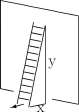
Example 8.4.1 A 10 meter ladder leans against a wall. The foot of the ladder slips horizontally at the rate of 1 meter per minute. At what rate does the top of the ladder descend when the top is 6 meters from the ground?
Draw a picture. See Figure 8.4.1.1. Let x be the distance from the wall to the foot of the ladder and let y be the distance from the ground to the top of the ladder. We are asked to find y’
CHAPTER 8. APPLICATIONS OF DERIVATIVES
376
at a certain instant. Because the top of the ladder is descending, we expect our answer (y f ) to be negative.
x and y are intrinsically related.
2 , 2
x + y
10 2
Figure for Example 8.4.1.1 Ladder leaning against a wall and sliding down the wall.
x and y are changing with time, and
(x(t)) 2 + (y(t)) 2 = 10 2 Differentiate with respect to t (use the chain rule, twice):
2x(t)x'(t) + 2y(t)y'(t) = 0
‘When’ The instant, to, specified in the problem is defined by y = 6. At that instant x 2 + 6 2 = 10 2 , so that x = 8. The problem also specifies x'(t) = 1 for all t. The actual value of t 0 is not required; we know that x(t 0 ) = 8, y(t 0 ) = 6, and x'(t 0 ) = 1. Therefore
(2 x 8 x 1) + (2 x 6 x y’) = 0
and y’ — — – meter/min
Example 8.4.2 In an aqueous solution the concentrations of H + and OH ions satisfy [H+] [OH-] = 1(T 14
If in a certain lake the pH is 6 ([H + ] = 1CT 6 ) and is decreasing at the rate of 0.1 pH units per year, at what rate is the hydroxyl concentration, [OH ], increasing?
Solution: It is useful to take the logw of the two sides of the previous equation:
log 10 ([ H+ ] [ OH- ]) = log 10 10
-14
log 10 [ H+] + log 10 [OH-] = -14
pH +log 10 [OH-] = -14
pH +
In [ OH-In 10
-14
CHAPTER 8. APPLICATIONS OF DERIVATIVES
377
Now we take derivatives of each term:
pH]’ +
In [0H-
[PH]’
In 10 [ OH” ] At the given instant, ( [ H+ ] = 106 ) so that
[KT 6 ] [ OH- ] = 1014 and [OH
Also, by the hypothesis, [pH]’ = —0.1. Therefore
In 10 OH-
[-14]’
10″
[pH]’ +
In 10 [ OH
-0.1 +
1
In 10 10″
1 OT\ S
[ [OH-] ]’ = 0.1 (In 10) 108 = 0.23 10~ 8 —per second
Example 8.4.3 In Exercise 7.3.7 we discussed the following problem.
A piston is linked by a 20 cm tie rod to a crank shaft which has a 5 cm radius of motion (see Figure 8.4.3.3). Let x(t) be the distance from the rotation center of the crank shaft to the end of the tie rod and 9(t) be the rotation angle of the crank shaft, measured from the line through the centers of the crank shaft and piston. The crank shaft is rotating at 100 revolutions per minute. The goal is to locate the point of the cylinder at which the piston speed is the greatest.
We present an analysis of this problem that illustrates some common steps in such problems.
Figure for Example 8.4.3.3 Crank shaft, tie rod, and piston (or fly rod, fly line, and fish).
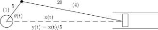
Step 1. We rescale the problem by dividing dimensions by 5. We are more accurate manipulating 1 and 5 than manipulating 4 and 20. Thus the parenthetical entries (1), (4), and (y(t) = x(t)/5) in Figure 8.4.3.3. Observe that 3 < y < 5.
By the Law of Cosines,
4 2 = l 2 + 2/ 2 (t) -2-1 x y(t)-cos6(t). (8.11) Differentiation of this equation yields
0 = 0 + 2y(t)y'(t) – 2y'(t) cos6(t) – 2y(t)(-sin0(t))0′(t)
CHAPTER 8. APPLICATIONS OF DERIVATIVES
378
y'(t) y(t) sinfl(t)
6′{t) cos9(t)-y(t)
y’it) y(t) sinfl(t)
200vr cos9(t) – y(t) :
(100 rotations per minute implies that 9′ = 2007r). From Equation 8.11
(8.12)
cos6> =
y -15
2y
and from sin 2 9 + cos 2 9 = 1 we find sin 9 = ±
A
1 –
y 2 -15\ 2
±
3<y<5,
4y 2 _ ( y 2 _ 15 )2
2y ; 2y
Now use Equation 8.12 to write y'(t) in terms of y(t), and suppress the (t).
3 < y < 5.
% 2 – (y 2 – 15) S
2007T
±-
2y
y -15
2j/
y y^y 4 + 3%2 _ 225
r+ 15
Note the change from ± to =p. Now to find the value of y for which y’ is maximum, we might wish to compute [y’\ = ^ ‘ and find where it is zero. Computation of [y’\ from the previous equation appears to be messy.
Step 2. Instead we note that where y’ is a maximum, [y’] 2 is also a maximum and we look at
Z [ 200vr J
y^J-y 4 + My 2 – 225 \ ‘ _ -y 6 + 3V – 225y 2
^ + 15
(y 2 + isy
This ratio of polynomials is easier to differentiate.
dz (y 2 + 15) 2 [ -y 6 + 3V – 225y 2 }’ – (-y 6 + 3% 4 – 225y 2 ) [ (y 2 + 15)-dy ~ (l/ 2 + 15) 4
-2y)
y 6 + 45y 4 – 1245y 2 + 3375
3 < y < 5
(y 2 + 15) 3
Explore 8.4.1 You should check the previous computation.
Step 3. We need to know the value of y for which z’ = 0. That will only occur when y = 0 (outside of 3 < y < 5) and when the numerator, y 6 + 45y 4 — 1245y 2 + 3375 = 0. It is helpful that the denominator is never zero. So solve
y 6 + 45y 4 – 1245y 2 + 3375 = 0
Clever Step 4. Only even powers of y occur in this sixth degree polynomial. Let w = y 2 and solve
CHAPTER 8. APPLICATIONS OF DERIVATIVES
379
Just as the roots to a quadratic equation are given by the formula — 2 — , there are formulas for the roots to cubics, but they are seldom useful. Instead we use a polynomial solver on a calculator and compute the roots
Wl = -64.96412 w 2 = 16.88784 w 3 = 3.07628
The root W2 = 16.88784 is relevant to our problem. We remember that w = y 2 and x = 5y and compute
y = V16.88784 = 4.10948 x = hy = 5 x 4.10948 = 20.55
From the dimensions of the crank shaft and tie rod, x is between 15 and 25. The highest speed of the piston occurs at x = 20.55, to the right of midpoint of its motion.
Exercises for Section 8.4 Related Rates
Exercise 8.4.1 A pebble dropped into a pond makes a circular wave that travels outward at a rate 0.4 meters per second. At what rate is the area of the circle increasing 2 seconds after the pebble strikes the pond?
Exercise 8.4.2 A boat is pulled toward a dock by a rope through a pulley that is 5 meters above the water. The rope is being pulled at a constant rate of 15 meters per minute. At the instant when the boat is 12 meters from the dock, how fast is the boat approaching the dock?
Exercise 8.4.3 Corn is conveyed up a belt at the rate of 10 m 3 per minute and dropped onto a conical pile. The height of the pile is equal to twice its radius. At what rate is the top of the pile increasing when the volume of the pile is 1000 m 3 ? (Note: Volume of a cone is \v:r 2 h where r is the radius of the base and h is the height of the cone.)
Exercise 8.4.4 A light house beacon makes one revolution every two minutes and shines a beam on a straight shore that is one kilometer from the light house. How fast is the beam of light moving along the shore when it is pointing toward the point of the shore closest to the light house? How fast is the beam of light moving along the shore when it is pointing toward a point that is one kilometer from the closest point of the shore to the light house?
Exercise 8.4.5 Two planes are traveling at the same altitude toward an airport. One plane is flying at 500 kilometers per hour from a position due North of the airport and the other plane is traveling at 300 kilometers per hour from a position due East of the airport. At what rate is the distance between the planes decreasing when the first plane is 8 km North of the airport and the second plane is 5 km East of the airport?
Exercise 8.4.6 Two planes are traveling at the same altitude toward an airport. One plane is flying at 500 kilometers per hour from a position 8 km due North of the airport and the other plane is traveling at 300 kilometers per hour from a position 5 km due East of the airport. Assuming the planes continue on a path over and beyond the airport, how long afterward and at what distance will the planes be the closest to each other?
CHAPTER 8. APPLICATIONS OF DERIVATIVES
380
Exercise 8.4.7 A woman 1.7 meters tall walks under a street light that is 10 meters above the ground. She is walking in a straight line at a rate of 30 meters per minute. How fast is the tip of her shadow moving when she is 5 meters beyond the street light?
Exercise 8.4.8 A gas in a perfectly insulated container and at constant temperature satisfies the gas law pv 1A = constant. When the pressure is 20 Newtons per cm 2 the volume is 3 liters. The gas is being compressed at the rate of 0.2 liters per minute. How fast is the pressure changing at the instant at which the volume is 2 liters?
Exercise 8.4.9 Find x’ at the instant that x — 2 if y’ — 5 and
a. xy + y = 9 b. xe y = 2e c. x 2 y + xy 2 = 2
Exercise 8.4.10 A point is moving along the parabola y = x 2 and its y coordinate increases at a constant rate of 2. At what rate is the distance from the point to (4,0) changing at the instant at which x = 2?
Exercise 8.4.11 Accept as true that if a particle moves along a graph of y = f(x) then the speed of the particle along the graph is \J(x’) 2 + (y’) 2 .
(The notation means that x’ is the rate at which the x-coordinate is increasing, y’ denotes the rate at which the y-coordinate is increasing and the speed of the particle is the rate at which the particle is moving along the curve.)
a. Suppose a particle moves along the graph of y = x 2 so that y’ = 2. What is x’ when y = 2? How fast is the particle moving?
b. Suppose a particle moves along the circle x 2 + y 2 = 1 so that its speed is 2n. Find x’ when x = l.
c. Suppose a particle moves along the circle x 2 + y 2 = 1 so that its speed is 2n. Find x’ when x = 0. (Two answers.)
8.5 Finding roots to f{x) = 0.
It is unfortunately frequent to encounter simple equations such as xe~ x = a for which no amount of algebraic manipulation yields a solution such as x = an expression in a. Three numerical schemes are commonly used to solve specific instances of such equations: iteration, the bisection method, and Newton’s method.
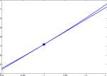
Example 8.5.1 Problem. Solve xe~ x = a for a = 0.2 and a = 2.
Solution. Graphs help explore the problem. Shown in Figure 8.10A is a graph of y = xe~ x . It is apparent that the highest point of the graph has y-coordinate about y = 0.37. We are relieved of solving xe~ x = 2; there is no solution. The dashed line at y = 0.2 does intersect the graph of y = xe~ x ; at two points so there are two solutions to xe~ x = 0.2, r\ at about x = 0.3 and r 2 at about x = 2.5.
Iteration. There is a simple scheme that sometimes works. xe~ x = 0.2 is equivalent to
x = 0.2e x . We can guess x 0 = 0.3 as an estimate of r±, and compute a new estimate
xi = 0.2e xo = 0.2e 0 3 = 0.2700. Then compute x 2 = 0.2e Xl = 0.2e a2700 = 0.2620. Continue and we find that
CHAPTER 8. APPLICATIONS OF DERIVATIVES
381
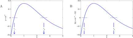
Figure 8.10: A. Graph of y = xe x . B.Graph of y = xe x — 0.2.
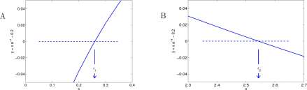
Figure 8.11: A. Graph of y = xe x — 0.2 on 0 < x < 0.4. B. Graph of y = xe x — 0.2 on 2.35 < x < 2.37.
Correct to four decimal places, x = 0.2592 is a solution to xe~ x = 0.2. This scheme fails for finding the root r 2 near x = 2.5 and an alternate scheme is suggested in Exercise 8.5.1.
The general pattern of this method is that you convert your problem of solving g(x) = 0 into a problem of solving x = f{x). Then you make a guess of Xq cis ctn approximation to the root, r, for which both g{r) = 0 and r = f(r). Then you compute X\ = f(x Q ), x 2 = x 3 = f(x 2 ), ■ • ■■ The
condition for this to succeed is that |/'(r)| < 1 and is reported in Theorem 14.4.1.
Iterations can be easily performed on a hand calculator that has an ‘ANS’ button, meaning, perform the previous step using the current answer on the screen. An example to solve x = 0.2 e~ x is
0.3 ENTER 0.2 * e”(-ANS) ENTER ENTER ENTER ENTER ENTER Produces .30000 .14816 .17246 .16832 .16902 .16890
The ‘-‘ sign is denotes ‘negative’ and not ‘subtraction.’
Another approach. It is common to modify the problem and examine the function,
f(x) = x ex – 0.2
the graph of which is shown in Figure 8.11B. We are searching for points where the graph of / crosses the x-axis (that is, f(x) = 0).
CHAPTER 8. APPLICATIONS OF DERIVATIVES
382
Bisection. A rather plodding, but sure way to find r\ is called the bisection method. We observe from Figure 8.11A that r\ appears to be between 0.2 and 0.3. We check
/(0.2) = .2 e’2 – .2 = -0.03625 and /(0.3) = .3 e” 3 – .2 = 0.22245
Because /(0.2) is negative and /(0.3) is positive, we think / should be zero somewhere between 0.2 and 0.3.
Next we check the value of / at the midpoint of [0.2, 0.3] and
/(0.25) = -0.0052998
Because /(0.25) is negative and /(0.3) is positive, we think / should be zero somewhere between 0.25 and 0.3.
Now we check the value of / at the midpoint of [0.25, 0.3] and
/(0.275) = 0.0088823
Because /(0.25) is negative and /(0.275) is positive, we think / should be zero somewhere between 0.25 and 0.275.
Obviously this can be continued as long as one has patience, and the interval containing the root decreases in length by a factor of 0.5 each step. Computation of seven decimal places in ri = 0.2591711 requires
0.1 x 0.5″ < 0.5 x 10⁻⁸ which implies that n > 24.25
or 25 steps.
Newton’s Method. It may not be a surprise to find that Isaac Newton, in the days of quill and parchment and look up table for trigonometric and exponential and logarithm functions functions 5 , developed a very efficient method for finding roots to equations. We suppose, as before, that a function, /, is defined on an interval, [a, 6], that for some number, r, in [a, b] f(r) = 0, and we are to compute an approximate value of r. It is also necessary to know the derivative, /’ of / (which Newton was also good at).
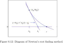
Newton began with an approximate value xq to r. Then he found the equation of the tangent to the graph of / at the point, (x 0 , f(x 0 )). He reasoned that the tangent was close to the graph of / and should cross the horizontal axis at a number, xi, close to r, where the graph of / crosses the axis. x\ is easy to compute, and is an approximate value to r. Newton repeated the process as necessary, but we will see that not many repetitions are required.
An equation of the tangent to the graph of / at the point (x 0 , f(x 0 )) is
V – ^ Xq) = f'(x 0 ) Equation of Tangent
X — Xq
The tangent crosses the horizontal axis at (x 1: 0). By substitution,
0 ~ f(x 0 ) Xi – x 0
We solve for x\ and find
Xi = X 0 –
= f(x 0 )
f(xo) f(x 0 )
5 Trigonometry has a long history and was well summarized by Claudius Ptolemy (ca 90 – ca 168 AD) in his ” Amalgamcst”; John Napier published “Minfici Logarithmum Canonis Descriptio” (Description of the Wonderful Rule of Logarithms) in 1614.
CHAPTER 8. APPLICATIONS OF DERIVATIVES
383
If we repeat this process, we will find a next approximation, x 2 to r, where
X 2 = X\
The general formula is
fix,
J\Xn) n -, 0
x 0 given x n+1 = x n – — —- n = 0,1, 2,
f (Xn)
In the special case,
f( x ) =xe~ x – 0.2 f{x) = e~ x – xe~ x
_ x n e~ x ” – 0.2
SO tllclt X n -\-i — X n
We choose xq = 0.3. Then
0 3 e -0 3 — 0 2 x x = 0.3 —— no ;„ = 0.25710251645
0 25710251645 e -o-257io25i645 _ q 9
a; 2 = 0.25710251645 nog ‘ nog1<8>lg n = 0.25916608777
z e -0.25710251645 _ q 25710251645 e -0 25710251645
A summary of the computations is shown in Table 8.1. The remarkable thing is that after only four iterations, we obtain 15 digit accuracy. It is typical that the number of correct digits doubles on each step (underlined digits). By contrast, the bisection gets one new correct digit in roughly three steps. The bisection method requires 48 steps for comparable accuracy.
It would not have escaped Newton that the iteration
x n e~ Xn – 0.2
Xn+1 = Xn ~ ~ ~~
can be simplified to
CHAPTER 8. APPLICATIONS OF DERIVATIVES
384
Table 8.1: Matlab program to compute Newton iterates to solve xe x — 0.2 = 0. The underlined digits are accurate and the number of accurate digits doubles with each iteration.
MATLAB program Output
close all ;clc; clear 0.300000000000000
format long 0.257102516450287
x=0.3 0.259166087769089
for k = 1:5 0. 25917110 1789536
x = x – (x – 0.2*exp(x))/(l-x); 0. 259171101819074
disp(x) 0.259171101819074
end
Newton’s method to solve f(x) = 0 requires three things. First it requires the derivative of /, but there is an alternate method that uses an average rate of change rather than the rate of change and works almost as well. Secondly, a good approximation to the root is required, and there is no substitute for that. Finally, in order to eliminate some unpleasant pathology, it is sufficient to assume that /, /’ and /” are continuous and that
m /» < !
(f(s)f
These conditions are often met. ■
Exercises for Section 8.5, Finding roots to f(x) = 0.
Exercise 8.5.1 Try to solve xe~ x = 0.2 by iteration of x n+ \ = 0.2e Xn beginning with xq = 2.5. This is easily done if your calculator has the ANS key. Enter 2.5. Then type 0.2 x e ANS , ENTER, ENTER, • • •. Describe the result. Try again with xq = 2.6. Describe the result. An alternate procedure is to solve for follows.
xe~ x = 0.2 0.2
e x = —
x
0.2
—x = in —
x
0.2
x — — In — = ln(5 x)
x
Now let x 0 = 2.5 and iterate x n+ \ = ln(5 x n ) and describe your results.
Exercise 8.5.2 Use a calculator that has the ANS key and compute the iterates of Equation 8.13, using xq = 0.3. Use
CHAPTER 8. APPLICATIONS OF DERIVATIVES
385
0.3 ENTER ANS – (ANS – 0.2*e”(ANS))/(1-ANS) ENTER ENTER ENTER
Exercise 8.5.3 Begin with x 0 = 0.25917110182 and compute the iteration steps (x n+ \ = x n e~ Xn — 0.2). Describe your results.
Exercise 8.5.4 Refer to Figure 8.11B and use the bisection method to find the root to f(x) = xe~ x — 0.2 near x = 2.5.
Exercise 8.5.5 Use three steps of both the bisection method and Newton’s method to find the a value s in the indicated interval for which f(s) = 0 for
a. f(x) = x 2 -2 [1,2] b. f( x )= x 3-5 [1,2]
c. f( x ) = x 2 + x – 1 [0,2] d. f(x) = (x – V2) 1/3 [0,1]
Exercise 8.5.6 Suppose you are trying to solve f(x) = 0 and for your first guess, Xo, f'(xo) = 0. Remember that x\ is defined to be the point where the tangent to / at (x 0 , f(xo)) intersects the X-axis. What, if anything, is x 1 in this case?
Exercise 8.5.7 (A common example.) Use Newton’s Method to find the root of
f(x) = x^
(Overlook the fact that the root is obviously 0!) Show that if x 0 — 1 the successive ‘approximations’ are 1, -2, 4, -8, 10, • • •.
Exercise 8.5.8 Ricker’s equation for population growth with proportional harvest is presented in Exercise 14.3.4 as
Pt+i -P t = aP t e-^f 3 -RP t If a fixed number is harvested each time period, the equation becomes
P t+1 -P t = aP t ePt/ ? – H
For the parameter values a = 1.2, (5 — 3 and H — 0.1, calculate the positive equilibrium value of P t .
8.6 Harvesting of whales.
The sei whale (pronounced ‘say’) is a well studied example of over exploitation of a natural resource. Because they were fast swimmers, not often found near shore, and usually sank when killed, they were not hunted until modern methods of hunting and processing at sea were developed. Reasonably accurate records of sei whale harvest have been kept. “• • -sei whale catches increased rapidly in the late 1950s and early 1960s (Mizroch et al., 1984c). The catch peaked in 1964 at over 20,000 sei whales, but by 1976 this number dropped to below 2,000 and the species received IWC protection in 1977.” http://spo.nwr.noaa.gov/mfr611/mfr6116.pdf
Data shown in Figure 8.13 are from Joseph Horwood, The Sei Whale: Population Biology, Ecology & Management, Croom Helm, London, 1987.
The International Convention for Regulating Whaling was convened in 1946 and gradually became a force so that by 1963/64 effective limits on catches of blue and fin whales were in place because of depletion of those populations. As is apparent from the data, whalers turned to the sei
CHAPTER 8. APPLICATIONS OF DERIVATIVES
386
o o
CfcP
o°o
Figure 8.13: Harvest of Sei whales, southern hemisphere, 1910 – 1979.
whale in 1964-65, catching 22,205 southern hemisphere sei whales. Catches declined in the years 1965-1979 despite continued effort to harvest them, indicating depletion of the southern hemisphere stock. A moratorium on sei whale harvest was established in 1979. The Maximum Sustainable Yield (MSY) is an important concept in population biology, being an amount that can be harvested without eliminating the population.
Explore 8.6.1 Would you estimate that the southern hemisphere sei whale would sustain a harvest of 6000 whales per year?
The actual size of a whale population is difficult to measure. A standard technique is the ‘Mark and Recapture Method’, in which a number, N, of the whales is marked at a certain time, and during a subsequent time interval the number m of marked whales among a total of M whales sited is recorded.
Exercise 8.6.1 Suppose 100 fish in a lake are caught, marked, and returned to the lake. Suppose that ten days later 100 fish are caught, among which 5 were marked. How many fish would you estimate were in the lake?
Another method to estimate population size is the ‘Catch per Unit Effort Method’, based on the number of whale caught per day of hunting. As the population decreases, the catch per day of hunting decreases.
In the Report of the International Whaling Commission (1978), J. R. Beddington refers to the following model of Sei whale populations.
N t+1 = 0.94N t + Ni
t-8
0.06 +0.0567 U
2.39^
0.94Q (8.14)
N t , N t+ i and N t s represent the adult female whale population subjected to whale harvesting in years t, t + 1, and t — 8, respectively. C% is the number of female whales harvested in year t. There is an assumption that whales reach sexual maturity and are able to reproduce at eight years of age
CHAPTER 8. APPLICATIONS OF DERIVATIVES
387
and become subject to harvesting the same year that they reach sexual maturity. The whales of age less than 8 years are not included in N t . N* is the number of female whales that the environment would support with no harvesting taking place.
Exercise 8.6.2 Show that if there is no harvest (C t = 0) and both N t and Af t _ 8 are equal to N* then N t+1 = N*.
If we divide all terms of Equation 8.14 by N*, we get
C t
N t +i N t N t _ t+i = n 94— H —
N* ^iV + TV*
, Nt. ^ 39 ~ 0.06 + 0.0567 U – ,
-0.94-
We might define new variables, D t — ^ and E t = j£- and have the equation
A+i = 0.94A + A-8 [0.06 + 0.0567 {l – ££?£}] – 0ME t (8.15)
Equation 8.15 is simpler by one parameter (iV*) than Equation 8.14 and yet illustrates the same dynamical properties. Rather than use new variables, it is customary to simply rewrite Equation 8.14 with new interpretations of N t and C t and obtain
N t+ i = 0.94N t + N t _ 8 [0.06 + 0.0567 {l – A^f}] – 0.94C t (8.16)
N t now is a fraction of N*, the number supported without harvest, and C t is a fraction of N* that is harvested.
Equation 8.14 says that the population in year t + 1 is affected by three things: the number of female whales in the previous year (N t ), the “recruitment” of eight year old female whales into the population subject to harvest, and the harvest during the previous year (C t ).
Exercise 8.6.3 a. Suppose iV* = 250, 000 and a quota of 500 female whales harvested each year is established. Change both Equations 8.14 and 8.16 to reflect these parameter values.
b. Suppose 2% of the adult female whale population is harvested each year. Change both Equations 8.14 and 8.16 to reflect this procedure.
c. What is the meaning of 0.94 at the two places it enters Equation 8.16? The term
N t _ 8 [0.06 + 0.0567 {l – (iV t _ 8 ) 2 39 }”
represents the number of eight year old females recruited into the adult population in year, t. The factor,
0.06 +0.0567{l – (iV t _ 8 ) 2 39 }”
represents the fecundity of the females in year t — 8. It has been observed that as whale numbers decrease, the fecundity increases. This term was empirically determined by Beddington.
Exercise 8.6.4 Draw the graph of fecundity vs N t s-
Exercise 8.6.5 Suppose harvest level, Ct is set at a constant level, C for a number of years. Then the whale population should reach an equilibrium level, N e , and approximately
JV t+ i = N t = Nts = N e
We would like to have N e as a function of the harvest level, C. This is a little messy (actually quite a bit messy), but it is rather easy to write the inverse function, C as a function of iV e .
CHAPTER 8. APPLICATIONS OF DERIVATIVES
388
a. Let C t — C and N t+l — N t — N t _ 8 = N e in Equation 8.16 and solve the resulting equation for C. Draw the graph of C vs N e .
b. Find a point on the graph of C(N e ) at which the tangent to the graph is horizontal.
c. If you did not do it in the previous step, compute C'(N e ) = J^- and find a value of N e for which C'(N e ) is zero.
d. Give an interpretation of the point (N e ,C(N e )) = (0.60001,0.025507). What do you suppose happens if the constant harvest level is set to C = 0.03?
e. N* for the southern hemisphere sei whale has been estimated to be 250,000. If N* is 250,000, what is the maximum harvest that will lead to equilibrium? You should find that the maximum supportable yield of the southern hemisphere sei whale is about 6000 whales per year.
Exercise 8.6.6 In this problem, you will gain some experience with the solution to Equation 8.16 for several values of the parameters. You should record the behavior of the solutions for different parameter values. You may wish to use the MATLAB program
close all;clc;clear
C=0.0255; S=0.61; iter = 150; space = 5 for k = 1:9 N(k)=S;
end
for k = 10:iter
N(k) = 0.94*N(k-1)+N(k-9)*(0.06+0.0567*(1-N(k-9)~(2.39)))-0.94*C;
end
N(10:space:iter)’
a. Run the program. What happens to the whale population?
b. Change S = 0.61 to S = 0.59, and run again. What happens to the whale population?
c. Change C = 0.0255 to C = 0.023 and run again. What happens to the whale population?
d. Find the values of N e that correspond to C — 0.023. Suggestion: a. Iterate x 0 = 0.5, x n+1 = 0.3813 + x 3 n 39 . b. Iterate x 0 = 0.5, x n+l = (x n – O.SSIS)^ 3 39 ).
e. Use C = 0.0230 and S = 0.43 and run again. What happens to the whale population?
f. Change S = 0.43 to S = 0.45 and run again. What happens to the whale population?
g. Change S = 0.45 to S = 0.78 and run again. What happens to the whale population?
8.7 Summary and review of Chapters 3 to 8.
Definitions. We have introduced the concepts of difference quotient of a function and rate of change of a function, and applied the concepts to polynomial, exponential and logarithm functions and trigonometric functions. The difference quotient of a function is:
Difference quotient of P on \a, b] = ^—— ^ Q
b — a
CHAPTER 8. APPLICATIONS OF DERIVATIVES
389
where P is a function whose domain contains at least the numbers a and b.
To compute the rate of change of P at a number a in the domain of P, we compute the difference quotient of P over intervals, [a, b], having a as one endpoint and decreasing in size to zero. Then there is that mysterious step of deciding what those difference quotients get close to as b gets close to a. Assuming the difference quotients get close to some number, that number is called the rate of change of P at a and is denoted by P'(a).
The symbol, P’, denotes the function defined by
P'{a) = the rate of change of P at a
for every number a in the domain for which the rate of change exists.
The words ‘get close to’ are sometimes replaced with ‘approaches’, and the word ‘limit’ is used for the number that (P(b) — P(a))/(b — a) gets close to. This can reduce a lot of words to a simple symbol,
P» = lim Pib lPia > (8.17)
b^a b – a
Chapter Exercise 8.7.1 Let P(t) = \ft and a be a positive number. Give reasons for the following steps to find P'(a).
P'(a) = lim —^ ^ (i)
b-+a b- a
r Vb-^
= lim — In)
b^a b – a
= lim (in)
b ^ a Vb + y/a
l _ l
(iv)
Chapter Exercise 8.7.2 Suppose P(t) = t A .
a. Write an expression for (P(b) — P(a))/(b — a), the difference quotient of P on the interval, [a, b].
b. Simplify your expression.
c. Use your simplified expression to show that the rate of change of P at a is 4 a 3 .
Chapter Exercise 8.7.3 Use the definition of rate of change to find the rate of change of P(t) = | at a = 5. Repeat for a unspecified. Complete the formula
P(t) = \ => P\t) =
The functions F and G of the next two exercises present interesting challenges. Chapter Exercise 8.7.4 Nine points of the graph of the function F defined by
F{£) = ^ for n=l,2,3,—
(8.18)
F(0) = 0
are shown in Chapter Exercise Figure 8.7.4a.
CHAPTER 8. APPLICATIONS OF DERIVATIVES
390
a. Plot two more points of the graph of F.
b. Does F'(0) exist?
c. Does the graph of F have a tangent at (0,0)? Your vote counts.
Figure for Chapter Exercise 8.7.4 Graphs of F and G for Chapter Exercises 8.7.4 and 8.7.5.
-0.6 -0.4 -0.2 0 0.2 0.4 0.6
-0.8 -0.6 -0.4 -0.2 0 0.2 0.4 0.6 0.8
Chapter Exercise 8.7.5 Nine points of the graph of the function G defined by
G
■iy
n
for n= 1,2,3,• • •
U9)
G(0) = 0
are shown in Chapter Exercise Figure 8.7.4b.
a. Plot two more points of the graph of G.
b. Does G'(0) exist?
c. Does the graph of G have a tangent at (0,0)? Your vote counts. 8.7.1 Derivative Formulas.
Using the definition of rate of change, we obtained formulas for derivatives of six functions.
Primary Formulas
[C]’
0
ct
c-1
(8.20) (8.21)
[In t}’ [sin t]’
1
t
cos t
$.23) 124)
= e f (8.22) [ cos t]’ = _ sint ( 8 . 2 5)
Then we obtained rules for derivatives of combinations of functions.
Combination Rules
[Cu(t)}’ = Cu'(t)
(8.26)
[u(t)+v(t)]’ = u'(t)+v'(t)
[u(t)v(t)}’ = u'(t)v(t)+u(t)v'(t)
~u(t)Y v{t) u it) – u{t) v’it)
W)\ ~ KO?
[G(u(t))]’ = G'(u(t))u'(t)
(8.27)
(8.28)
(8.29)
(8.30)
Formula 8.30, ([G(u(t))\ = G'(u(t)) u'(t), called the chain rule) is a bit difficult for students, and special cases were presented.
Chain Rule Special Cases
ran/
[(«(*)) ,u(t)
pn( «(*))]’ M «(*))]’
n (w(t)) n_1 u'(t) e u(t) u'(i)
«(*)
cos( -u(t)) u'(t)
(8.31) (8.32) (8.33) (8.34)
[cos( «(*))]’ = -am(u(t))u'(t)
(8.35)
One special case of the chain rule is so important to the biological sciences that it requires individual attention.
e kt k = k e kt
(8.36)
Example 8.7.1 Usually more than one derivative formula may be used in a single step toward computing a derivative. It is important to know which steps are being used, and a slow but sure way to insure proper use is to use but a single formula for each step. We illustrate with
CHAPTER 8. APPLICATIONS OF DERIVATIVES P(t) = \e t2 + e
392
P'(t) =
= 4
= 4 = 4 = 4
e* + sin t
e* + sint
e + sint
e + sint
e* + sint
e* + sint
e* + sin t
+ [sint]’
(e* 2 [t 2 ]’ + [sint]’) (e* 2 (2t) + [sint]’) (e* 2 (2t) + cost
Notational identity. Equation 8.31 Equation 8.27
Equation 8.32 Equation 8.21 Equation 8.24.
Observe that the the first three steps used combination formulas; the last two steps involved primary formulas. A common pattern.
Chapter Exercise 8.7.6 Use the derivative formulas, one formula for each step, to find P'(t) for
Chapter Exercise 8.7.7 Compute the derivatives of a. P{t) = t 5 + 3t 4 -4t 2 + l
c. P(t) = t 4 e*
e. P{t) = ^ g- Pit)
g 3£ g 5t
b. Pit) = t3
d. Pit) = (t + e*) 4
f. Pit) = ln(t 2 + l)
CHAPTER 8. APPLICATIONS OF DERIVATIVES
393
Chapter Exercise 8.7.8 The word differentiate means ‘find the derivative of. Differentiate
8.7.2 Applications of the derivative
Geometry. The rate of change of P(t) at a is the slope of the tangent to the graph of P at the point (a, P(a)). With only one exception, the existence of a tangent to the graph of P at (a, -P(a)) is equivalent to the existence of the rate of change of P(t) at a. The exception is illustrated by
Chapter Exercise 8.7.9 Let P(t) = U.
a. Draw the graph ofPon— 1 <t < 1.
b. Draw the tangent to the graph of P at (0,0).
c. For (a,P(a)) = (0,0), compute (P(b) – P{a))/{b – a).
d. Discuss lim^o (P(b) – P(0))/(6 – 0).
Chapter Exercise 8.7.10 Find an equation of the line tangent to the graph of P(t) = e* at the point (1, e 1 ) = (1, e).
The tangent line lies close to the graph near the point of tangency, and is often used as an easily computable approximation to the graph. The next problem illustrates this.
Chapter Exercise 8.7.11 In Problem 8.7.10 you found the equation of the line tangent to the graph of P{t) = e t at the point (l,e). Let y x denote the y-coordinate of the point on the tangent whose x-coordinate is x.
a. Find y L8 .
b. Compute e LS .
c. Compute the relative error
d. Mark the points (1.8,P(1.8)) and (1.8, yi. 8 ) on a copy of the graph in Figure 8.7.11A.
e. Find y 1A .
CHAPTER 8. APPLICATIONS OF DERIVATIVES
394
g. Compute the relative error
Via ~ e
1.1
h. Mark the points (1.1,P(1.1)) and (l.l,yx.i) on a copy of the graph in Figure 8.7.11B. Figure for Chapter Exercise 8.7.11 Graphs of y = e x and its tangent at (l,e) at two scales.
A ^ ■ ■ ■ ^ B
Chapter Exercise 8.7.12 Let P(t) = t 3 + 6t 2 + 9t + 5. Find the intervals on which P'(t) > 0. If you draw the graph of P on your calculator, you will observe that P is increasing on these same intervals.
Chapter Exercise 8.7.13 Find an equation of the line tangent to the graph of P(t) = t 3 — 3t 2 + 5 at the point (1,3). Find a point on the graph of P at which the tangent to the graph is horizontal.
8.7.3 Differential Equations
With each of the derivative formulas we found equations involving those derivatives (called differential equations) that describe dynamics of some biological systems.
Chapter Exercise 8.7.14 We will find in Chapter 17 that a population of size, P(t), growing in a limited environment of size, M, is modeled by an equation of the form
P'(t) = k P{t) and that P(t) can be written explicitly as
P(t)
M
P 0 Me
ki
kt
M-P 0 + P 0 e
where Pq is the population size at time t — 0. Assume P 0 = 1, M = 10, and k = 0.1.
a. Use the first equation and draw a graph of P 1 vs P.
b. What value of P maximizes P’l
c. Use the second equation and draw the graph of P(t).
d. Draw a tangent to the graph of P at the point for which P’ is a maximum. Is the point an inflection point?
CHAPTER 8. APPLICATIONS OF DERIVATIVES
395
e. Rewrite your equation to be
^) = S ^ T T = io(^ 0 ” + i)” 1
and compute P'(t).
f. At what time t and population size, P(t), is P'(t) a maximum?
Chapter Exercise 8.7.15 Heavy rainfall in the drainage area of a lake causes runoff into the lake at the rate of 100e~* acre-feet per day. The accumulated runoff into the lake due to the rain after t days is 100(1 — e *) acre feet. Water is released from the lake at the rate of 20 acre-feet per day and the volume of the lake at the time of the rain was 400 acre-feet. Flood stage is 450 acre-feet.
a. Write an equation for the volume, V(t) of water in the lake at time t days after the rain, accounting for the initial volume, the volume accumulated due to the rain, and the total volume released during the t days.
b. Does the lake flood?
c. At what time does the lake reach its maximum volume and what is the maximum volume?
Chapter Exercise 8.7.16 This exercise explores the optimum clutch size for a bird. Most biological parameters are compromise values that optimize some feature of the system. In this model, we assert that clutch size of birds is adapted to maximize the number of birds that survive for three months past hatching. The data is for a chickadee, Parus major, as observed in woods near Oxford, England 6 . This is part of a historic study of the chickadee population in those woods begun in 1947 and from which data are still being gathered. Only two of the several factors influencing clutch size are considered here, the weight, WT of the young at age 15 days in a clutch of size n, and the percent of fledglings recovered 3 months past fledging. The data is for the year 1961. In order to have several young survive to age three months, a large clutch should be produced. However, if the clutch is too large the adults can not adequately feed the young, they are small at fledging, and the probability of survival is reduced. The following exercises explore the relations between the parameters.
The basic data is displayed in Chapter Exercise Figure 8.7.16 along with the following parabolas that approximate the data:
WT = -0.024(5/} – 3.25) 2 + 19.2 (8.37)
PCT = 0.75(W-15) 2 (8.38)
WT is the average weight at 15 days of chicks in a clutch of size BD, and PCT is the percent of chicks of weight W at 15 days that survive to 90 days.
Figure for Chapter Exercise 8.7.16 Data and quadratic approximations for chickadees. A. Graph of average body weight vs clutch size. B. Graph of percent survival to 90 days vs body weight of chick. WT = -0.024(55 – 3.25) 2 + 19.2 and PCT = 0.75(W – 15) 2 .
6 C. M. Perrins, Population fluctuations and clutch-size in the great tit, PARUS MAJOR L., J. Animal Ecol. 34 601-647 (1965)
CHAPTER 8. APPLICATIONS OF DERIVATIVES
396
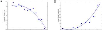
Clutch size Weight at 15 days – gm
We make an assumption that the expected number, XP, of chicks that survive to age 90 days from a clutch size of BD is
XP = BD PCT/100. (8.39)
The distribution of weights of chicks at 15 days within a clutch is unknown to us; we are assuming that W = WT, an assumption we would prefer to avoid.
a. Assume that W = WT and use Equations 8.37 and 8.38 to write a single equation for PCT in terms of BD.
b. Now use Equation 8.39 to write XP in terms of BD.
c. Use simpler notation.
y = x 0.0075 x 0.024 2 [(x – 3.25) 2 – 175] 2 Use derivative formulas to compute y’.
d. One factor of y’ is 5x 2 — 19.5x — 164.4375. Find a value of x between 6 and 10 for which y'(x) = 0.
e. How many chicks from a brood of optimum size would be expected to survive?
You should have found that a clutch size of 8.0 will maximize the expected number of chicks that will survive to 90 days. From table 14 of Perrins, 383 broods had an average brood size of 8.1 chicks.
Chapter 9
The Integral
9.1 Areas of Irregular Regions. Area of an oak leaf.
Explore 9.1.1 Describe two ways to approximate the area of the leaf shown in Figure 9.1. ■
You may think of several interesting ways of solving the previous problem. A way that we will generalize to future applications is illustrated by two problems following Figure 9.1.
One of the more curious ways of estimating the area of the leaf in Figure 9.1 is to paste the page on a dart board and throw darts at the page from a distance sufficient to insure that the points where the dart hits the page are randomly distributed on the page. The number, Np, of darts that strike the page and the number, Nl, of darts that strike the leaf can be counted. The area of the leaf is approximated by
N L
Area of the leaf = —— Area of the page.
N P
Although the procedure may seem a bit esoteric, it is used in serious computations of volumes in high dimension (with points randomly generated by a computer algorithm rather than darts!).
CHAPTER 9. THE INTEGRAL
398

Figure 9.1: An Oak leaf.
CHAPTER 9. THE INTEGRAL
399
Explore 9.1.2 The darker grid lines in Figure 9.2 are marked at 1.0 cm intervals. Count the number I\ of 1.0 cm 2 squares entirely covered by the leaf and the number 0\ of 1.0 cm 2 squares that intersect the leaf (including those included in 7i). Use I\ and 0\ to estimate the area of the leaf. ■
The finer grid on the leaf in Figure 9.2 is marked at 0.5 cm intervals. We count that 1 2 = 283 of these squares are completely inside the leaf and a total of O2 = 409 squares intersect the leaf (not including the stem). Because each square is of area 0.25 cm 2 the area of the leaf should be at least 283 x 0.25 = 70.75 cm 2 and no more than 409 x 0.25 = 102.25 cm 2 .
Explore 9.1.3 How do 70.75 and 102.25 cm 2 compare with your answer based on the 1 cm 2 squares? Given the information so far obtained, what is your best estimate of the area of the leaf? How can you extend the procedure to get an even better answer? ■
Let A denote the area of the leaf in Figure 9.2. Because the area of each 1cm grid square is lcm 2 , Ii x 1 is the area of the region covered by the the 1cm grid squares inside the leaf, and /[ x 1 is less than A. Because the squares that intersect the leaf enclose the leaf, 0\ x 1 is greater than A.
Explore 9.1.4 Because every 1-cm square inside the leaf contains four 0.5-cm squares also inside the leaf,
h x 1.0 < I 2 x 0.25.
Explain why
a. I 2 x 0.25 < A < 0 2 x 0.25 b. 0 2 x 0.25 < d x 1.0. ■
The normal distribution. Shown in Figure 9.3 is (a portion of) the graph of the probability density function of the normal distribution, sometimes called the ‘Bell-shaped curve’. In the figure shown, the distribution has mean zero and standard deviation equal to one. The equation of the density function is
1 _s£
f (x) = —1= e 2 _ oo < x < 00 (9.1)
The interpretation of the density function is that if a measurement of a sample from a normal variate has been scaled so that the average value is zero and the standard deviation is one, then for any interval [a, b] of measurement values, the probability that any one member of the sample lies in [a, b] is the area of the region between x = a and x = b and below the curve and above the horizontal axis. The area under the total curve, from —00 to +00, is 1.0. The graph is symmetrical about the Y-axis, so that, for example, the area to the left of the vertical axis is equal to the area to the right of the vertical axis, the two areas sum to one, and therefore both areas are 0.5.
The normal distribution is important because many biological measurements (heights of European women, lengths of ears of a certain variety of corn) are approximately normally distributed about their means. Such quantities are thought to be essentially the sum of a large number of independent small quantities (determined by genetic factors that have additive effects), which would account for the cumulative effect being normally distributed. Also, for any distribution, the means of repeated samples from the distribution are approximately normally distributed. For example, if you randomly select 50 people from a given population and compute the mean of their heights, and repeat this experiment 100 times, then the 100 means so computed will be approximately normally distributed.
CHAPTER 9. THE INTEGRAL
400
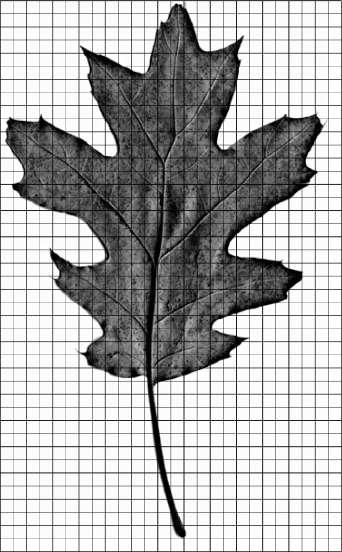
Figure 9.2: An Oak leaf with 1cm and 0.5cm grids.
CHAPTER 9. THE INTEGRAL
401
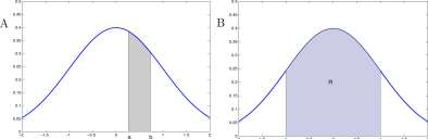
Figure 9.3: A. A graph of a portion of the particular normal distribution that has mean zero and standard deviation one, Equation 9.1, f(x) = _/= e~ x / 2 . The probability that a number drawn from this normal distribution lies in the interval [a, b] is the area of the shaded region below the graph and above [a, b]. B. The shaded region, R, is bounded by the graph of the normal distribution, the X-axis, and the vertical lines x — — 1 and x — 1.
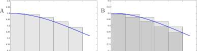
Figure 9.4: Graphs of the normal distribution density function, f(x) = -^^ e ~ x2 ^ 2 i between x = 0 and x = 1. A. Upper rectangle approximation to the area between the graph of the curve and the X-axis and the lines x = 0 and x = 1. B. Same as A with lower rectangles included.
Example 9.1.1 Problem: Find (approximately) the area of the region R in Figure 9.3B bounded by the graph of the normal distribution, /, the X-axis, the vertical line, x = — 1 and the vertical line, x = 1. Solution:
1. Because of the symmetry of the region R about the F-axis, it is sufficient to find the area of that portion of R that is to the right of the F-axis, and then to multiply by 2. The portion R to the right of the F-axis is shown in Figure 9.4A.
2. Compute the sum of the areas of the upper rectangles in Figure 9.4A. The width of each rectangle is 0.2 and the heights of the rectangles are determined by the density function, f. The area of the leftmost rectangle, based on the X interval [0, 0.2], is
/(0) x 0.2 = ^=e-^ x 0.2 = 0.079788 v 2tt
CHAPTER 9. THE INTEGRAL
402
The area of the second rectangle from the left, based on the X interval [0.2, 0.4], is
1 2
/(0.2) x 0.2 = -—e” 2 *” x 0.2 = 0.078209 v 2ir
Explore 9.1.5 Find the areas of the remaining three rectangles in Figure 9.4A. ■
3. The sum of the areas of the five rectangles is 0.356234; twice the sum is 0.712469. This is an over estimate of the area of R.
4. An under estimate of the area can be computed by summing the areas of the lower rectangles in Figure 9.4B. The leftmost lower rectangle, based on the X interval [0, 0.2] has the same area as the second upper rectangle from the left, based on the X interval [0.2,0.4], and we computed that area to be 0.078209. The next three rectangles are similarly related to upper rectangles, and their areas are precisely the areas you computed in the preceding problem.
The area of the right most lower rectangle is
x 0.2 = 0.07358
‘2tt
and the sum of the five areas is 0.324840; twice the sum is 0.649680.
5. We now know that the area of R, is greater than 0.649680 and less than 0.712469. A good estimate of the area of R is the average of these two bounds,
0.649680 + 0.712469
= 0.681075.
2
The probability of being within one standard deviation of the mean in a normal distribution is 0.68268949 correct to eight digits.
Ozone: The Alfred Wegner Institute Foundation for Polar and Marine Research, Bremerhaven Germany, has measured (among a large number of interesting things) ozone partial pressures at altitudes up to 35,000 meters since March 1992 at their Georg von Neumayer research Station in the Antarctic. Two relevant web sites are:
http://www.awi-bremerhaven.de/
http: / / www.awi. de/en/infrastructure / stations / neumayer ^station / observatories/meteorologicaLobservatory /upper _air .soundings/ozone .soundings/
Color graphs at the site show the ozone history since 1992. An image for 2004 is shown in Figure 9.5. Data read from that graph for the ozone partial pressure as a function of altitude on day 100 is shown in Table 9.1.
Assume that the “ozone layer” lies between 14 and 28 kilometers, and that the density of the ozone is proportional to the partial pressure (which would be OK were the temperature constant). We ask, how much ozone is in the ‘ozone layer’ on day 100 above the Neumayer station? More specifically, we assume that the density of ozone in grams per kilometer cubed is a constant, K, times the partial pressure of ozone and ask how much ozone is in a column that is above a 100
CHAPTER 9. THE INTEGRAL
403
Neumayer Radiosonde Station 70 s 39 1 South. &” 15 r West Oeone Partial Pressure (nanobar)
I I I I I i I i i I > I i I i I i I ‘ I I I I I II I I I I I I I 1111| |i| i| || 11| ill ll i| 1414 I I III II I I I I
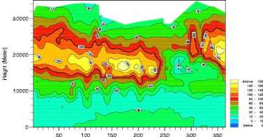
Day of Year 2004
Figure 9.5: Ozone partial pressure at the Neumayer Station.
Table 9.1: Data read from Figure 9.5 for day 100.
28 26 24
20 1 8 1 6 1 4
CHAPTER 9. THE INTEGRAL
404
meters (=0.1 km) by 100 meters square that surrounds the Neumayer antarctic station and between the altitudes 14 and 28 kilometers (see the diagram in Table 9.1).
Consider first that portion, Pi, of the column between 14 and 16 km. The volume of Pi is
0.1×0.1×2 km 3 = 0.02 km 3
The ozone density at 14 km is K x 60 and at 16 km is K x 90 gm/km 3 . We assume that the average density for all of Pi is the average of K x 60 and K x 90, or K x 75 gm/km 3 . Then the mass of ozone in Pi is calculated as
Mass of ozone in Pi = 0.02 km 3 x K x 75 gm/km 3 = K x 1.5 gm
Similarly we calculate the mass of ozone in the portion, P 2 , of the column:
Mass of ozone in P 2 = 0.02 km 3 x K x ^ + jjj gm/km 3 = K x 2.05 gm
Continuing we get the mass of ozone in the section of the column above Neumayer station to be 13.7 K gm.
Exercises for Section 9.1, Areas of Irregular Regions.
Exercise 9.1.1 Find (approximately) the area of the region in Figure 9.3 bounded by the graph of the normal distribution, /, the X-axis, the vertical line, x = — 2 and the vertical line, x — 2.
Because we found the area of the region R bounded by x = — 1 and x — 1 you might reasonably conclude that your main task is to find the area of the region bounded by the graph of the normal distribution, the X-axis, the lines x — 1 and x — 2. Then add some numbers.
You should find that the probability of being within two standard deviations of the mean of the normal distribution is approximately 0.95 (the probability is 0.95449974 correct to eight digits).
Exercise 9.1.2 Shown in Figure 9.6A are the hourly readings for solar radiation intensity for June 21, 2004 recorded by the University of Oregon Solar Radiation Monitors Laboratory at their station in Eugene, Oregon (http://solardat.uoregon.edu). The data are for ‘global irradiance’ which includes all radiation falling on a horizontal plate measured in watts/meter 2 .
The data in Figure 9.6A shows that, for example, at 10 am the solar intensity was 780 w/m 2 on June 21, 2004 in Eugene, Oregon. If the solar intensity were constant at that value from, say, 9:30 am to 10:30 am, then the energy that would fall on a 1 meter 2 panel during that time would be 780 w-hr. This is the area of the rectangle encompassing 10 am in Figure 9.6A. The solar energy striking aim 2 panel during the whole day is approximately the sum of the areas of the rectangles shown in Figure 9.6B.
a. How many watt-hours of energy struck a 1 meter 2 panel at Eugene, Oregon on June 21, 2004?
b. What is the value of that amount of energy at $0.08 per kilowatt-hour?
Exercise 9.1.3 Shown in Figure 9.1.3 is a graph of the average daily solar intensity for Eugene, Oregon plotted as a function of day number, 1 < day < 365. (The average is for the years 1990 -2004, except for 2001 for which no data are posted.)
CHAPTER 9. THE INTEGRAL
405
A
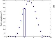
Time of day, June 21, 2004
Time ol day, June 21, 2004
Figure 9.6: A graph of the solar intensity at Eugene, Oregon for June 21, 2004 (http://solardat.uoregon.edu). The measure is global irradiance which is the total energy striking a horizontal plate measured in watts/meter 2 .
a. Was the sun intensity on June 21, 2004 above or below average for June 21 according to your answer to Exercise 9.1.2
b. Use the graph in Figure 9.1.3 to compute in two different ways the total energy and the value of the total energy striking a one meter square panel for one year at Eugene, Oregon.
1. Partition the year into 6 60-day intervals plus a single 5-day interval. Use as the solar intensity the average of the highest and lowest energies for that interval.
2. Partition the year into 12 30-day intervals plus a single 5-day interval. Use as the solar intensity for each interval the average of the solar intensities at the first and last days of the interval.
c. At $0.08 per kw-hr, what is the value of the average solar energy that struck a one meter square panel for one year at Eugene, Oregon?
Figure for Exercise 9.1.3 A graph of the average solar intensity at Eugene, Oregon as a
function of day of year.
8
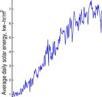
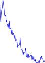
0
0
30
60
90
120
150
180 210 2
Day of year
240
270
300
330
360
Exercise 9.1.4 Dr. Frank Vignola of the University of Oregon forwarded the following practical problem. Pixels in satellite images are used to estimate solar irradiance values. The satellite images are taken at 15 minutes after the hour and the users need hourly values. How would one estimate hourly values from the data obtained at 15 minutes after the hour and how are the data degraded when the data are shifted?
Exercise 9.1.5 a. Using the data shown in Figure 9.1.3, let E(t) be the cumulative energy striking a one meter-square panel from day one to day t. Compute E(30), £(60), £(90), £(120), £(150), and £(180).
b. Plot your data.
c. Estimate £(135) and £(140) from your data.
d. At (approximately) what rate is E(t) increasing at time t = 135?
Exercise 9.1.6 a. Draw a horizontal line on Figure 9.1.3 so that the area of the rectangle
bounded above by your horizontal line and below by the t-axis on the left by the vertical axis, t = 0 and on the right by the vertical line t = 365 is the same (approximately) as the area under the solar intensity curve (Figure 9.1.3).
b. Where does your line cross the vertical axis?
c. On what days does your line cross the curve?
d. What is the average daily solar intensity for the year?
Exercise 9.1.7 Compute the mass of ozone in the layer between 14 and 28 km above the 0.1 km square surrounding the Neumayer station for days 150 and 280. It may be easier to read the color graph at http://www.awi-bremerhaven.de/MET/, search for ‘ozone 2004.’ At what time of year is there ‘a hole in the ozone?’
CHAPTER 9. THE INTEGRAL
407
Monte Carlo Integration. Although as noted we will not make serious use of Monte Carlo integration (throwing darts at pictures of leaves), you may find the next three exercises interesting and they may add to your understanding of ‘area’.
Exercise 9.1.8 Decide what will be meaning of the output of the program in Exercise Figure 9.1.8. (It is written for MATLAB, but very similar language is used for calculators and other computer programs).
Figure for Exercise 9.1.8 A MATLAB program. A collection of 100 points randomly
distributed in a square with sides of length 1.
close all;clc N=100; count=0; for i = 1:N
x(i) = rand; y(i) = rand;
if x(i)~2 + y(i)~2 < 1 count = count+1;
end
end
plot(x,y,’x’,’linewidth’,2) axis([0 1 0 1] ,’square’) set(gca,’xtick’,[0 0.2 0.4 0.6 0.8 1.0] set(gca,’ytick’,[0 0.2 0.4 0.6 0.8 1.0] 4*count 0.2
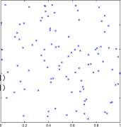
Exercise 9.1.9 Modify the previous program to estimate the area of the ellipse
2 2
x y
— + — = 1
25 9
Exercise 9.1.10 Modify the previous program to estimate the area of the region bounded by the graphs of
1
y = ,— e 2 , y — 0, x — 0, and x — 1
Exercise 9.1.11 If an object moves at a constant speed, s m/min, over a time interval [a, b] minutes, the distance, D, traveled is D = s m/min x(b — a) min, D = s x [b — a) meters.
If the speed s(t) varies over [a,b], the distance, D, can be approximated by partitioning [a, b] by a = to < t% < • • • < t n -i <t n = b into n subintervals so that s(t) is approximately constant on each subinterval 1 . Then D is the sum of the distances traveled during each subinterval and
D = s(tx) x (tx – t 0 ) + s(t 2 ) x (t 2 — tx) H h s{t n ) x (t n – i n _ x ) meters.
CHAPTER 9. THE INTEGRAL
408
Approximate the distance traveled by a particle moving at the following speeds and over the indicated time intervals. Partition each time interval into 5 subintervals.
a. s(t) = t on 1<{<6 b. s(t) = t 2 on 0<i<2
c. s(t) = l/t on 1 < t < 3 d. s(t) = y/i on 2<t<7
Exercise 9.1.12 Problem: What is the mass of a column of air above a one-meter square table top?
Imagine a one meter square vertical column, C, of air starting at sea level and extending upwards to 40,000 meters.
Shown in Figure 9.1.12 are ‘standard’ values of atmospheric density as a function of altitude up to 40,000 meters (U.S. Standard Atmospheres 1976, National Oceanic and Atmospheric Administration, NASA, U.S. Air Force, Washington, D.C. October 1976). The density is not constant throughout C, and the mass of C may be approximated by partitioning C into regions of ‘small’ volume, assuming that the density is constant within each region, and approximating the mass within each of the regions. Then the object will approximately have
Mass = 5i x vi + 62 x v 2 + ■ ■ ■ + 5 n x v n where 5k Kg/m 3 and Vk m 3 are respectively the density and volume in the kth region.
a. Partition the altitude interval from 0 to 40,000 meters into at least 6 subintervals (they need not be all the same length). For each interval, find the volume of the region of C corresponding to the interval, find a density of the air within that region, and approximate the mass of the region. Approximate the mass in each region and add the results to approximate the mass of air in C.
b. Does the size of your answer surprise you? Show that it is consistent with the standard pressure of one atmosphere being 760 mm of mercury? The density of mercury is
1.36 x 10 4 Kg/m 3 .
Figure for Exercise 9.1.12 Air density at various altitudes up to 40,000 meters. The horizontal segments are intended to assist in reading data from the graph.
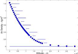
CHAPTER 9. THE INTEGRAL
9.2 Areas Under Some Algebraic Curves
409
In This Section
Formulas are developed for the area of the region bounded by the t-axis, the graphs of y = t n , t = 0, and t = x for n = 0, 1, 2, and 3. The result is that: The area of the region bounded by the t-axis and the graph of y = t n between t = 0 and t = x is
v n+l
11
for n = 1, 2, 3, and 4. The formula is actually valid for all values of n except n = — 1.
A = x 1 /1
y=t°
A = x /3

t = x
A = x /2

t = x
A = x /4

t = x
The work of this section requires some arithmetic formulas. Let n be a positive integer.
1 + 1 + 1 + — + 1
n
n terms
1 + 2 + 3
l 2 + 2 2 + 3 2
l 3 + 2 3 + ■ ■ ■ + n a
n
n
n(n + 1)
n(n + 1) (2n + 1) 6
n 2 (n + l) 2
(9.2) (9.3) (9.4) (9.5)
Explore 9.2.1 Do this.
a. Run the following MATLAB program and interpret the results.
clear x
for i = 1:10; x(i)=i”2; end; x sum(x)
b. Alternate. Execute the following commands on your calculator and interpret the result. seq(k~2,k,1,5)
sum seq(k~2,k,1,5)
and interpret the results. Note: sum and seq can be found in the menu 2nd LIST OPS
c. Check that l 2 + 2 2 + 3 2 + • • • + n 2 = n(w+1) 6 (2 ” +1) is valid for n = 10 and n = 5000.
d. Check that
n x (n + 1)
is valid for n = 100. 2
Equations 9.2 – 9.5 and many similar equations are proved by the method of Mathematical Induction that is described in Appendix A.
Example 9.2.1 Problem. Find the area of the region R illustrated in Example Figure 9.2.1.1A that is bounded by the parabola y = t 2 , the t-axis, and the line t = x where a; is a positive number.
Figure for Example 9.2.1.1 A. The region R bounded by the parabola y = t 2 , the t-axis, and the line t = x. B. The same parabola with n rectangles with bases in [0, x\.
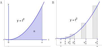
Solution. The sum of the areas of the rectangles in Figure 9.2.LIB approximates the area of R. The interval [0, x] on the horizontal axis has been partitioned into n subintervals by the numbers
0, 2- ••• (n-1)-, n-
n n n n
The width of each rectangle in the figure is -. The height of each rectangle is the height of the parabola y = t 2 at the right end of the base of the rectangle. The heights of the rectangles, from left to right, are
(£hjg’ – (<»-^) 2 . (+o 2
2 Carl F. Gauss’s fourth grade teacher assigned his class the task of computing 1 + 2 + • • • 99 + 100 (probably to keep the little rascals busy for a while). Young Carl quickly responded, 5050, and explained that 1 + 2 + • • • 99 + 100 = (1 + 100) + (2 + 99) + ••• (50+51) = 50 x 101 = 5050. Note that 50 x 101 = lSOxioi_ Tq Mg credit] the teacher promptly recognized genius, and brought Gauss to the attention of the local nobleman.
CHAPTER 9. THE INTEGRAL
411
The sum, U n , of the areas of the rectangles is
” \nJ n \ nj n V n J n \ nJ n
;i 2 + 2 2 + — + (n-l) 2 + n 2 )4
71/
(9.6)
2ra 3 + 3n 2 + n * 6>? X
3 + + 6^) x3
This is powerful medicine. The region R covered with n = 50 rectangles is illustrated in Figure 9.2.1.1C. The sum of the areas of the fifty rectangles, U50, is close to the area of R, and
U 50 = ( l + —— + ——j”) x 3 = f 1 +0.01 + 0.000067) x 3 = l x 3 50 V3 2 x 50 6 x 50 2 / V 3 ; 3
lim U n = lim —I 1 ^ ) x
n^oo n-+oo \% 2n 6n
11 1\ , x 3
Furthermore,
In Section 9.4 the area of R is defined to be this limit, so that:
For the region R bounded by the parabola y = t 2 , the i-axis, and the line
t — x,
x 3
the area of R is —. (9.7)
Figure for Example 9.2.1.1 (Continued) C. The parabola of A with 50 rectangles with bases in
[0,1].
c
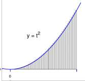
CHAPTER 9. THE INTEGRAL
412
Upper rectangle approximation
Lower rectangle approximation
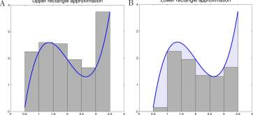
Figure 9.7: A. Upper rectangles approximating the area of a region bounded above by the graph of a function, /. B. Lower rectangles approximating the area of the same region.
Upper and lower rectangles. Note we freely use summation symbols such as
E k2
k=l
and
n-l
E
k=0
Explanation of this notation is included in Appendix A.
In the Example 9.2.1 the top edges of the approximating rectangles were entirely on or above the graph of y = t 2 and are called upper rectangles and their sum, f/ 50; is an upper approximation to the area under consideration, as shown in Figure 9.7A. When the top edges of the rectangles lie entirely on or below the graph, the rectangles are called lower rectangles and their sum is called a lower approximation, as shown in Figure 9.7B. The area of the region lies between the upper and lower approximations.
Example 9.2.2 Problem. Find approximately the area of the region R illustrated in Example Figure 9.2.2.2A bounded by the cubic y = x 2 (2 — x), and the X-axis.
Figure for Example 9.2.2.2 A. The region R bounded by the cubic y = x 2 (2 — x) and the X-axis B. The same cubic with 10 rectangles with bases in [0,2].
A
B
CHAPTER 9. THE INTEGRAL
413
The cubic y = x 2 (2 — x) = 2x 2 — x 3 intersects the x-axis at x = 0 and x — 2. The rectangles in Figure 9.2.2.2 partition [0,2] into ten intervals and the sum of the areas of the rectangles approximates the area of the region R. The rectangles are a mixture of lower and upper rectangles. The base of each rectangle is 0.2 and its height is the height of the left edge. For k — 0 to 9, the height of the k + 1st rectangle, [k x 0.2, (k + 1) x 0.2], is 2 x (k x 0.2) 3 – (k x 0.2) 2 . The area of the /c + 1st rectangle is
2 x (jfe x 0.2) 2 – (k x 0.2) 3 ] x 0.2 The sum of the areas of the rectangles is
a
Y, [ 2 x (/c x 0.2) 2 -(h 0.2) 3
fe=0 9
£ [2(0.2) 2 x A; 3 – (0.2) 3 x k 2
x 0.2
x 0.2 =
fc=0
2(0.2) 3 ]T k 3 -(0.2) 4 ^k 2
fc=0 fc=0
2(0.2)
3 9(9 + 1)(2 x 9 + 1)
(0.2)
4 9 2 (9 + l) 2
= 1.32
Exercises for Section 9.2, Areas Under Some Algebraic Curves.
Exercise 9.2.1 Use Mathematical Induction as shown in Appendix A to show the validity of Equation 9.3
n(n + 1)
l + 2 + 3 + — + n= — -. Exercise 9.2.2 Show the validity of Equation 9.5
l 3 + 2 3 + 3 3 + • • • + n a =
3 _n 2 (n + l) 2
Exercise 9.2.3 Find the generic terms for the following sums, and write the sums using E notation.
a. 2 2 + 4 2 + 6 2 + 8 2 + 10 2
c.
d.
c.
u ‘ 1.1 ~ 1.2 ~ 1.3 ~ 1.4 ~ 1.5 ~ 1.6 ~ 1.7 ~ 1.8 ~ 1.9 ~
X
10
(-1.0) 3 + (-0.9) 3 + (-0.8) 3 + + ••• + (-0.2) 3 + (-0.1) 3 ] x ^ VI – 0.1 2 + Vi – 0.2 2 + VI – 0.3 2 + • • • + VI – 0.9 2 + Vi -1-0 2
x
CHAPTER 9. THE INTEGRAL
414
Exercise 9.2.4 Give reasons for
a.
Exercise 9.2.5 Evaluate:
a – Efc=i k b. Efe=3 ^
e- E^ 2 f. £
100 7,3 fc=3 ft
n(n — 1) 2
n(n + l)(2n + 1) 6
r V 100 h
L – Z^fc=18 ft
-1
d. Efc=i 2A;
h. E£ 0 5 o(3A; + 7)
i. El° =1 5A; 2 j. E^° 3 (A;3-9) k. Y.Z^k 2 – k) 1. (e^o 3*) + 7
Exercise 9.2.6 See Exercise Figure 9.2.6. Show that the lower approximation to the area of the region bounded by the graph of y = x 2 , the a;-axis, and the line x = 1 based on 10 equal subintervals is: a.
9
E
fc=0
10
1
To
9 x 10 x 19 1
x —-
6 10 3
c. The same as the upper sum minus the area of the tenth rectangle in the upper sum.
Figure for Exercise 9.2.6 Lower sum rectangles approximating the area of the region bounded
by y = x 2 , y = 0 and x = 1.
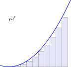
-0.2 0 0.2 0.4 0.6 0.8 1 1.2
Exercise 9.2.7 a. Find a formula for the sum, L n , of n lower rectangles approximating the area of the parabolic region, i?, of Figure 9.2.1.1A.
CHAPTER 9. THE INTEGRAL
415
c. Evaluate L 50 .
d. Evaluate lim^oo L n .
Exercise 9.2.8 Let R be the region bounded by the graph of y = t 3 , the t-axis, and the line t = x. See Figure 9.2.8
a. Write a formula for an upper sum, U n , of areas of n rectangles that approximates the area of R.
b. Condense U n into a single term as was done in Equations 9.6 for U n of the parabolic region.
c. Find lim U n .
n— >oo
Figure for Exercise 9.2.8 The region bounded by y — t 3 , the t-axis, and the line t — x
approximated by n rectangles.
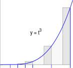
t = x
XXX X X
0 2 3 k n
n n n n n
0 X
Exercise 9.2.9 Compute the area of the region bounded by the graph of y = t 2 , the i-axis, and the lines t — 1 and t = 2. (Hint: Use Equation 9.7 and skip the rectangle bit.)
Exercise 9.2.10 Shown in Figure 9.2.10 is the first quadrant portion of the graph of x 2 + y 2 = 1.
a. Use x 2 + y 2 = 1 to compute the height of the fourth rectangle from the left.
b. Compute the area of the fourth rectangle from the left.
c. Write (do not evaluate) an expression for, £7 10 , that is the sum of the areas of the ten rectangles.
d. Write an expression for U\oo that is the sum of the areas of 100 rectangles that approximates the area of the quarter circle.
e. Use your computer or calculator to compute Uiqo and compare it with 7r/4.
CHAPTER 9. THE INTEGRAL
Figure for Exercise 9.2.10 The first quarter portion of the circle x 2 + y 2 =
416
1 and 10 rectangles.
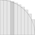
0 0.2 0.4 0.6 0.8
Exercise 9.2.11 Use ordinary geometry to
a. Show that the area of the shaded region in Figure 9.2.11A is x.
2
b. Show that the area of the shaded region in Figure 9.2.11B is
Figure for Exercise 9.2.11 A. Graphs of y = 1 and t = x. B. Graphs of y = t and t = x.
A
B 35
-0.5 0 0.5 1 1.5 2 2.5 3 3.5 4
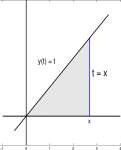
Exercise 9.2.12 A consequence of some previous problems is:
If n is either 0, 1, 2, or 3, £ is a positive number, and A is the area of the region bounded by the graphs of
y = t n y = 0 t = 0 and t = x,
then
Case : n = 0 A = x
Case : n = 1 A
Case : n = 2 A = ^
Case : n = 3 A Make a guess as to the values of A for n = 4, n = 10, and n = 1, 568.
x 2 ~2~
x 4 4
(9.
CHAPTER 9. THE INTEGRAL
417
Exercise 9.2.13 Summary Exercise: For additional practice on the preceding procedures, the following formula is presented.
n(n + l)(2n + l)(3n 2 + 3n – 1) 30
Use the formula to find the area of the region bounded by the graphs of
y = t 4 y = 0 t = 0 and t = x.
a. Suppose n is a positive integer. Partition [0, x] into n nonoverlapping intervals with end points
x x 0-2-n n
(Jfe-l)- k-n n
x
n-
n
b. What is the area of a rectangle based on the k th interval and having base interval,
((*-!)*(*;*) and height
k-
c. Show that the sum, U n , of the areas of all such rectangles is
X ° X – +
1 1
1
1
5 2n 3n 2 30n 4
d. Show that
lim U n
x
9.3 A general procedure for computing areas.
We generalize from the previous problems and define a procedure for computing the area of a region, R, bounded above by the graph of a function, /, below by the horizontal axis, on the left by a line t = a and on the right by a line t = b. The function, /, should be defined and positive for all t in [a,b]. We will assume / is increasing on [a, b]. Bounds on the errors of our estimates will be obtained.
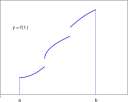
Assume / is a positive increasing function defined on an interval [a, b}. We describe a procedure to compute the area of the region between the graph of / and the X-axis as illustrated in Figure 9.8A. The function / may have one or more discontinuities. The region should be considered as the union of the vertical segments reaching from the horizontal axis to a point on the graph of /.
We can approximate the area of the region R as follows:
• Choose a number, n, of rectangles to be used.
• Let h = b -=±.
CHAPTER 9. THE INTEGRAL
418
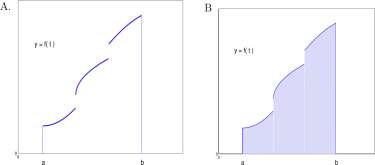
Figure 9.8: A. A region bounded above by the graph of an increasing function. B. Shaded region showing relation to discontinuities.
• Partition the interval [a, b] into n equal subintervals using points
a = t 0 < t\ < t 2 < ■ ■ ■ t n -\,t n = b. Because the intervals are of equal length, the length of each will be = h and
n
t 0 = a t\ = a + h t 2 = a + 2 x h ••• tj. = a + (k) X h ••• t n = a + n x h
• For k — 1, • • •, n, let be the area of the rectangle i^-i < t < t^, 0 < y < /(tfe). The rectangles are illustrated in Figure 9.9A and are referred to as upper rectangles.
• Let U n = J2k=i Ak- The union of the upper rectangles contains the region R so that U n is greater than or equal to the area of R.
• For k = 1, • • •, n, let be the area of the rectangle < t < t^, 0 < y < f{tk-\)- The rectangles are illustrated in Figure 9.9B and are referred to as lower rectangles.
• Let L n = Y^k=i Bk- The region R contains the union of the lower rectangles so that L n is less than or equal to the area of R.
For increasing functions
n n
L n=J2 X (** ~ and U n = £ /(**) X (** – tk-l)
k=l k=l
Shown in Figure 9.10 are both lower and upper rectangles approximating the area of the region R. The differences, A^ — B^, between the areas of the upper and lower rectangles are the areas of the small rectangles at the top of the larger rectangles. Copies of the small rectangles, translated horizontally, are shown in an “Error Box” to the right in Figure 9.10, and all are above an interval of width The height of the Error Box is vertical span of /, f(b) — f(a) and the
The Area of the Error Box is [/(&) ~ f( a )] x
Because
n n n
Un — L n — A h — B k — A k — B k
k=l k=l k=l
CHAPTER
9. THE INTEGRAL
419
A
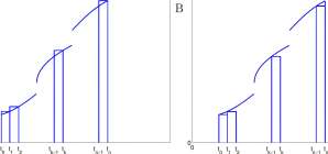
Figure 9.9: A. Upper rectangles for a region bounded above by the graph of a function. B. Lower rectangles for a region bounded above by the graph of an increasing function.
it follows that U n — L n is the area of the Error Box, or
U n – L n = [f(b) – f(a)) x b —^ (9.9) Equation 9.9 is important. Because
L n < The Exact Area of the Region R < U n
the approximation error in using either L n or U n as an approximation to the Area of R is no bigger than U n — L n . By choosing n large enough,
U n -L n = { f(b) – f(a) ) x —
n
can be made as small as one wishes and thus the error in using either U n or L n as an approximation to the Area of R can be made as small as one wishes.
Example 9.3.1 The previous information may be used in two ways, as illustrated in the following example.
1. First, one may have computed the upper approximating sum to the area of the region bounded by the graphs of y = s/i, y = 0, and t = 4 using 20 subintervals, as shown in Figure 9.3.1.1. The upper sum is 5.51557- ■ ■. The error box for this computation is shown to the right of the region. Because each rectangle is of width = 0.2, the error box is of width
0.2. The height of the error box is \fi — \/0 = 2 so the error in the approximation, 5.51557 ■ ■ ■ is no larger than 2 * 0.2 = 0.4.
2. On the other hand, one may wish to compute the area of the region in Figure 9.3.1.1 correct to 0.01, and need to know how many intervals are required to insure that accuracy. For any number, n, of intervals,
The error box is of height \/4 — Vo = 2 and width
n
CHAPTER 9. THE INTEGRAL
420
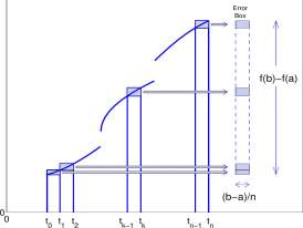
n-1 n
Figure 9.10: Upper and lower rectangles for a region bounded above by the graph of an increasing function.
Thus,
The size of the error box is
2 x
4-0
n n
Because the error is sure to be less than the size of the error box, our desired accuracy will be obtained if the size of the error box is less than 0.01. Therefore we require ^ < 0.01 so that
Q
qq^ < n, or n = 800. We will find that the actual error is only approximately one-half the size of the error box, and that n = 400 will almost give the required accuracy. ■
Figure for Example 9.3.1.1 The graph of y = yfx on [0,4] with 20 upper rectangles.
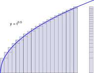
0 0.5 1 1.5 2 2.5 3 3.5 4 4.5 5
9.3.1 Trapezoidal approximation.
The average,
T
CHAPTER 9. THE INTEGRAL
421
often gives a very good approximation to the Area of R, and for increasing functions its error is less than | x (f(b) — /(a)) x (b — a) (one half the error of U n or L n ). For an evenly spaced partition of
[a, b],
b — a
tk — tk-1 = = h
and
and
n
U n = J2 f( f k) Xh aIld L n = J2 /(Vl) X h
fc=l fc=l
tt , r i / n n N
^ z \fc=i fc=i /
For the twenty intervals in Figure 9.3.1.1,
C/ 20 = 5.51557, L 20 = 5.11557,
(9.10)
and T 2 n = 5.31557.
The actual area is 5.33333 so that the error in T20 is 0.018, considerably less than the error bound for U20 of 0.4 computed in Example 9.3.1 and the actual error in {7 2 o °f 0.18.
The word trapezoid is used for T n because the average of the areas of the upper and lower rectangles
f{tk){tk – t k – 1) + f{t k -i)(tk – t k -i]
f(t k ) + f(t k -i)
(tk — tk-i)
is the area of the trapezoid, shaded in Figure 9.11, bounded on the left by the line from (£&_]., 0) to (tfc-i,/(tk_i)) and on the right by (t fc ,0) to (t k J(t k )).
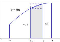
Figure 9.11: An increasing function. The average of the areas of the upper and lower rectangle is the area of the trapezoid.
CHAPTER 9. THE INTEGRAL
422
Example 9.3.2 Work done in compressing air. Movement a distance d (meters) against a constant force F Newtons 3 requires an amount W = F x d Newton-meters of work. If the force is not constant, the interval of motion [a,b] may be partitioned by
a = Xq < x 1 < x 2 < ■ ■ ■ < x n _i < x n = b.
If the force on interval [x k ^i,x k ] is approximately F k , then the work done is approximately
n
W = Yl F k X ( X k -X k -{). k=l
A 60 cc syringe was attached to a pressure gauge as shown in Figure 9.12. The plunger of area 5.5 cm 2 was extracted to 60 cc and the air inside the cylinder was at standard atmospheric pressure of Po — 760 mm mercury = 10.13 Newton/cm 2 . The plunger was pushed inward at 5 cc increments (to the 55 cc mark, to 50 cc, • • • to 20 cc and to 15 cc) and the pressure was recorded at each step (table in Figure 9.12). The distance between 5 cc marks on the syringe was 0.9 cm. Problem. How much work was done?
Solution. The force against the plunger on the fc th step was
F k = (P k – P 0 ) N/cm 2 x 5.5 cm 2 . The total work done, W, was approximately
9
W = ^(P fc -Po) N/cm 2 x 5.5 cm 2 x(i fc -xn) cm (9.11)
k=l 9
= Yl ( P * ~ P o) x 5.5 x 0.9 N-cm
k=l
Using the data from Figure 9.12 we calculate
W = 383 N-cm = 3.83 N-m
The number 5.5cm 2 x 0.9 cm is, except for measurement error, equal to 4.95 = 5 cm 3 , or the 5 ml marked on the syringe and in the data. Therefore the work done is
9 9
W = E ” P o) x (F fc _! – V k ) = -J2 ( p k – Po) x (V k – V k ^) N-cm (9.12)
k=l k=l
Continued in Exercise 9.3.13. One Newton-meter (called a Joule) is equal to 1 watt-sec. a flashlight with a 1.5 amp bulb and two 1.5 volt batteries uses 4.5 watts. The 3.83 N-m would burn the flashlight for 3.83/4.5 = 0.85 seconds. At $0.08 per kilowatt-hour, the value of the 3.83 N-m is $0.000000022. ■
Exercises for Section 9.3, A general procedure for computing areas.
Exercise 9.3.1 a. Identify two rectangles in Figure 9.10 whose areas are [/(ii) — /(*o)] x h. 3 N is the symbol for one Newton, the force required to accelerate 1 kilogram 1 meter per second per second.
CHAPTER 9. THE INTEGRAL
423
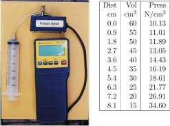
Figure 9.12: Syringe with attached pressure gauge and CBL manufactured by Vernier, Inc. Data from compressing the air in the syringe.
b. Identify two rectangles in Figure 9.10 whose areas are [ffo) — f{ti)] x h.
c. Identify two rectangles in Figure 9.10 whose areas are [/(£&) — f(tk-x)\ x h.
d. Identify one rectangle whose area is [/(&) — f(a)] x h.
Exercise 9.3.2 Suppose one is to compute the area of the region bounded by the graphs of
4
y = ;— o y = o t = o t = i y i + t 2 y
The graph of y = – 2 iS shown in exercise Figure 9.3.2. The graph is decreasing instead of 1 ~\-1
increasing, but with modest changes the Error Box computation still applies. The upper rectangles have the heights associated with the left ends of the intervals, and the lower rectangles have heights associated with the right ends of the intervals.
Figure for Exercise 9.3.2 The graph of y = 1/(1 + t 2 ).
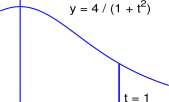
o 1 1 t
_11 1 1 1 1
-0.5 0 0.5 1 1.5 2
CHAPTER 9. THE INTEGRAL
424
Copy the picture to your paper and on your copy:
a. Shade the region bounded by the graphs of y — – 2 , V — 0, t — 0 and t — 1.
L ~\-1
b. Draw the upper rectangles based on n = 5 intervals.
c.
The upper sum based on n = 5 intervals is
4 4 4 4 4 1
= 3.334926
l + (0/5) 2 1 + (1/5) 2 l + (2/5) 2 1 + (3/5) 2 l + (4/5) 2 J 5
Draw the lower sum rectangles based on n = 5 intervals and compute the lower sum.
d. Draw the Error Box for the difference between the upper and lower sums based on n = 5 intervals. What is the area of the Error Box
e. Argue that for any n, U n — L n < 2/n.
f. What value of n should be chosen to insure that U n — L n < 0.004
g. Compute the upper and lower sums for n = 500. It was not terribly exciting to compute the lower sum for n — 5, and the computation for n = 500 may be a drag. Therefore, to compute the upper sum, run the following MATLAB program.
close all;clc;clear for k = 0:499
F(k+1)=( 4/(l+(k/500)~2) )/500;
end
U = sum(F)
L = U – 4/500 + 2/500 A = ( U + L )/2
Alternate. Enter the following strokes on your calculator:
sum seq(4/(l+(K/500)~ 2)*(l/500) ,K,0,499,1) ENTER Remember: sum and seq can be found in the menu
2nd LIST OPS
Your answer should be 3.143591987. Now press 2nd ENTER and modify the strokes to compute the lower sum.
h. What is your best estimate of the area based on L 50 o and ^soo-
i. The actual area of the region in question is ir = 3.141592654 • • •. Check that L 500 < ir < U 500 and that U 500 — L 500 = 0.004.
Exercise 9.3.3 Define a region that has area computed by
499
4 1
E
l + ((A; + 0.5)/500) 2 500′
k=0
CHAPTER 9. THE INTEGRAL
425
Exercise 9.3.4 Modify the MATLAB program or calculator steps shown in Exercise 9.3.2 and compute the sum of:
a. Forty rectangles to approximate the area of the region bounded by y = t 2 , y = 0, t = 2, and t = 4.
b. Forty rectangles to approximate the area of the region bounded by y = t 2 , y = 0, t = 1, and t = 5.
c. Forty rectangles to approximate the area of the region bounded by y = t 3 , y = 0, t — 1, and t = 5.
d. Forty rectangles to approximate the area of the region bounded by y — t -1 , y — 0, t — 1, and t — 5.
Exercise 9.3.5 Consider the region, R, bounded by the graphs of
y = l/t y = 0 t = 1 t = 2
See Exercise Figure 9.3.5. Into how many intervals of equal size must [1,2] be partitioned in order that the lower approximating rectangles will approximate the area of R correct to 3 decimal places (Error less than 0.0005).
Compute that sum on your computer or calculator. ( See methods in Exercise 9.3.2. ) It is a curious fact that the exact answer is In 2.
Figure for Exercise 9.3.5 The graph of y — 1/t.
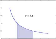
0 0.5 1 1.5 2 2.5 3 3.5
Exercise 9.3.6 Find a lower sum approximating the area bounded by the graphs of y = \/l — t 2 , y = 0, and t = 0 correct to 3 decimal places (error < 0.0005). What is the exact area?
Exercise 9.3.7 Compute the sum of the areas of 10 trapezoids based on the partition [0, 0.1, 0.2, • • •, 1] of [0,1] used to approximate the area of the region bounded by the graphs of
4
y = o y = o t = o t = l
y l + 1 2 y
Show that this sum more closely approximates the exact area than does the sum of 500 lower rectangles. The exact area is n.
Note: Be clever. Either use the average of upper and lower sums based on 10 intervals which have been previously computed, or use Equation 9.10.
CHAPTER 9. THE INTEGRAL 426 Figure for Exercise 9.3.7 Graph of y — 4/(1 + x 2 ), 0 < x < 1 for Exercise 9.3.7
Exercise 9.3.8 In Problem 9.3.5 you found that 1000 equal intervals are necessary in order that the rectangular sums approximating the area of the region bounded by the graphs of
y = l/t y = 0 t = l t = 2
approximate the area of the region correct to three digits (error less than 0.005). The area of the region correct to six digits is In 2 = 0.693147. Approximate the area of the region using 20 trapezoids based on equal subintervals of [1,2] and show that the accuracy of the approximation is better than that of the rectangular approximation using 1000 intervals.
Exercise 9.3.9 The exact area of the region bounded by the graphs of
y = Vt y = 0 and t = 5
is |5 3 / 2 = 7.453560. Compute the upper rectangular approximation and the trapezoidal approximation to the area based on 50 subintervals and compute their relative accuracies.
Exercise 9.3.10 Compute the area of the region bounded by the graphs of y = sinx and y = 0 for 0 < x < 7r using eight intervals and the trapezoid rule and the same eight intervals with upper rectangles. The exact answer is 2. Compute the errors and relative errors for each rule.
Exercise 9.3.11 Cardiac Stroke Volume. The chart in Figure 9.13 shows the timing of events in the cardiac cycle
a. Find a graph from which you can compute the ‘Aortic blood flow (ventricular outflow)’ measured in Liters/min.
b. The stroke volume may also be defined as the difference in the volume of blood in the ventricle at the end of diastole and the volume of blood in the ventricle at the end of systole. Find the curve ‘Ventricular Volume’, compute stroke volume from it, and compare with your previous computation.
c. Assume that one cardiac cycle takes about 0.8 seconds so that the heart is beating at 60/0.8 = 75 beats per minute.
Multiply the stroke volume for a single beat by 75 and compare with the conventional 5-6 Liters/minute for a resting adult.
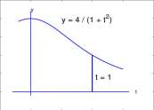
CHAPTER 9. THE INTEGRAL
427
i
EkM ol’JjTilL
^■iitrirticji
■ r 3 -t! Jr
Diimh-.i
L30 n
Anrtrpniwir
^■HUIlCillltpHilUt
Figure 9.13: A Wikipedia graph is shown: created by Agateller (Anthony Atkielski), converted to svg by atom. http://en.wikipedia.org/wiki/Electrocardiography Assume that the time from beginning of systole to the end of diastole is 0.8 seconds.
CHAPTER 9. THE INTEGRAL
428
Exercise 9.3.12 External Cardiac Work. This problem is directed to measuring the work done by the heart referred to as external work.
If liquid is pumped through a tube at a constant flow rate, R cm 3 /sec and at a constant pressure, P Newtons/cm 2 , during a time interval, [a, b] measured in seconds, then the work done, W, is
W = R x P x (b — a) Newton-cm.
a. Confirm that the units on R x P x (b — a) are Newton-cm, units of work.
b. Suppose the flow rate or pressure is not constant. Suppose R and P are continuous functions and the flow rate is R(t) and the pressure is P(t) for a < t < b. Let
a = t 0 < ti < t 2 < ■ ■ ■ < t n = b
be a partition of [a, b}. Write an approximation to the work, W, of pumping the liquid at the flow rate R(t) and pressure P(t) during [a, b] based on the partition.
c. The graph shown does not show Aortic blood flow. It does show, however, Ventricular volume which decreases during Systole. Use Ventricular volume to compute Aortic blood flow in ml/sec at 7 different points during Systole.
d. Using the same 7 points and read Ventricular pressure during Systole, and approximate the work done by a single stroke of the heart.
A much larger amount of work is done by the heart as ‘Internal Work’ that ‘includes transporting ions across membranes, internal mechanical events • • •, overcoming internal viscosity, and rearranging the muscular architecture as the heart contracts 4 ‘. Heart efficiency is defined as the ratio of External Work to the sum of External and Internal Work and ranges from 5 to 10 percent.
Exercise 9.3.13 Continuation of Example 9.3.2, Work done in compressing air.
a. Plot Pressure vs Volume for the data of Figure 9.12 and draw a smooth curve through the data points. Recall Equation 9.12. Interpret the work done, Equation 9.11, in terms of an area of that graph. Should the work done be positive?
b. It should be apparent from your graph and Equation 9.11 that we have computed (383 N-cm) an upper sum for the area. Compute a lower sum. Remember that for an increasing graph the lower sum is the upper sum minus the area of the error box. This is a decreasing graph. Try the same thing in this case.
c. Compute the average of the upper sum and lower sum. This is the trapezoidal approximation to the work done.
d. In 1662, Robert Boyle spread a rumor that PV = constant. But there is a 15% variation in PV shown in Table 9.2 and only 3.3% variation in P ■ {V + 3.6). Should we advise Boyle of his error, or examine our equipment?
Exercise 9.3.14 A tank has 30 m 3 capacity and has 15 m 3 of water in it. Water flows into it at the rate of R(t) = 1 + t 2 m 3 / min for 0 < t < 3 minutes. Does the tank overflow?
CHAPTER 9. THE INTEGRAL
429
Table 9.2: PV and P ■ (V + 3.6) for the data in Figure 9.12. PV 608 606 595 587 577 567 558 544 538 519
P(V + 3.Q) 644 645 637 634 629 625 625 623 635 643
Exercise 9.3.15 Records of Mississippi River discharge rates measured at McGregor, Iowa for April 16 – 22, 1994 are shown in the Exercise Table 9.3.15. Obtained from
http://co.water.usgs.gov/sediment/st...on_id=05389500 Note from the records that the flow increased and the sediment increased during that week, and it is reasonable to assume that there was a warm spell the led to snow melting or a rain in the drainage basin.
a. Approximate the total flow for the Mississippi for the week April 16 -22, 1994.
b. Approximate the total suspended sediment that flowed past McGregor, Iowa in the Mississippi River for the week of April 16-24, 1994.
c. The drainage basin is about 67,500 mi 2 . How many tons per square mile were removed from the drainage basin during that week?
Table for Exercise 9.3.15 Mississippi River Discharge, April 16-22, 1994.
Exercise 9.3.16 Work against the force of gravity. Suppose a 3 kilogram mass instrument is lifted 20,000 kilometers above the surface of the Earth, the force acting on it is not constant throughout the motion. See Figure 9.14. The acceleration of gravity may be computed for a distance x above the Earth as
R 2
Acceleration of gravity at altitude x = 9.8 x — — (9.13)
(R + x) 2 v 1
where R = 6,370 kilometers is the radius of the Earth. We partition the interval [0, 20,000] into 4 equal subintervals and assume the acceleration of gravity to be constant on each of the subintervals.
We introduce a new procedure: Choose the value of the acceleration of gravity for each subinterval to be the value at the midpoint of the interval. Thus the midpoint of the first interval, [0, 5000] is 2500 and the gravity constant for the first 5000 kilometers of motion will be
6370 2
9.8 x = 5.05
CHAPTER 9. THE INTEGRAL
430
; — x=2o,ooo
*
! x=15,000
x=10,000
x=5,000

x=0
Earth
Figure 9.14: Earth and a 3 kg object lifted 20,000 km above the surface.
The work to lift the instrument the first 5000 kilometers is approximately
5.05 x 3 x 5000
75814
Newton-meters
a. Approximate the total work to lift the instrument to 20,000 km.
b. Approximate the total work done to lift the 3 kg instrument 40,000 km. (You already know the work required to lift it 20,000 km.)
c. Approximate the total work done to lift the 3 kg instrument 100,000 km.
It is a very interesting question as to whether the instrument can ‘escape from the Earth’s gravity field’ with a finite amount of work. We will return to the question in Section 11.5.1, Escape Velocity.
We have used upper and lower rectangles to approximate areas between the graphs of functions and the horizontal axis. Other rectangular sums often give better estimates, but in most cases rectangular sums give acceptable estimates. In addition to areas, the approximating sums approximate other important physical and biological quantities, generally representing the accumulation of some quantity that is occurring at a variable rate. Implicit in all of the examples is that better approximations will be computed when the total interval is partitioned into smaller intervals. The total accumulation is called the integral of a function / on an interval [a, b]. A short definition of the integral is
9.4 The Integral
CHAPTER 9. THE INTEGRAL
431
Definition 9.4.1 The integral of a function, I. Suppose / is a function defined on an interval [a, b}. The integral of / from a to b is
lim
k=l
( b-a\ b-a f a + k x I x
n
n
if the limit exists. The notation for the integral is
rb
J a
or as in most calculus books
rb
/ /(*)
J a
dt
The function, /, is called the integrand, and
£
k=i
( b-a\ b-a f a + k x I x
n
n
(9.14)
is called an approximating sum for the integral.
Definition 9.4.1 is a formalization of the computations of the previous sections. The lim
n^oo
provides for the better approximations with smaller intervals in the partitions. The numbers
{b — a\ a \ b — a 6 — a b — a b — a 1 a + KX > = < a, aH , a H , •••a + k , ■■■,a + n = b } n J fc=Q [ n n n n J
partition [a, b] into n equal subintervals of length f(a + k x ^) evaluates / at the right endpoint of the kth interval.
±f(a + k , b -^), b -^ H I n ; n
sums the value of / at the right endpoint times the length of the interval. After discussion of notation, we will apply Definition 9.4.1 to relatively more difficult functions than we have considered so far.
Concerning the notations, J b a f and J b a f(t)dt.
The dt in J b f(t) dt is often a mystery to students, for good reason. The two notations for an integral in Definition 9.4.1 can be compared as follows. For f(t)=t 2 1 < t < 3, one may write
3
J f or one may write J t 2 dt
In a sense, j x t dt allows one to define the integrand f(t) = t and write the integral, all with one symbol. However, / x 3 t 2 would do that as well, so what is the dt! One could try to avoid the central problem by discussing
[ 3 e^dt Jo
and say that dt specifies that t is the independent variable (and not k). In fact,
dt is read ‘with respect to t.’
CHAPTER 9. THE INTEGRAL
432
The symbol f b f(t) dt is read, ‘the integral from a to b of / of t with respect to Furthermore, if you use a calculator or computer calculus package to compute J 0 3 e kt dt you have to specify that the integration is with respect to t (and not with respect to k). For example, with 100 stored in K on a TI-86, the command fnInt(K*x~2,x,0,1) returns 33.33. fnlnt(K*x~2,K,0,1) returns 4.9348 which is a bit of a mystery until you learn that 7r has been stored in x. The ‘respect to,’ (dt), is stored in the second position of fnlnt.
We will also find that dt is useful for keeping track of symbols in a change of variable in the integrand, and in doing so, dt is sometimes called a ‘differential.’
But there is a very colorful and controversial history of the symbol dt. We discuss it in the context of area. According to some, dt is an infinitesimal length on the t-axis, fit) dt is an infinitesimal area under the graph of /, and J b fit) dt sums the infinitesimal areas under the graph of / from a to b to give the total area under the graph of / between a and b. We will not attempt an elaboration. Many people use such intuitive language to quickly move from a physical problem to an integral that computes the solution to the physical problem. For example, if P(v) is the pressure in a syringe when the volume is v, then P(v) dv is the ‘infinitesimal work’ done when the plunger is moved and ‘infinitesimal distance’, dx, and the volume changes by an ‘infinitesimal volume’, dv, and the total work done in moving from v = 60 to v = 20 is / 60 P(v) dv.
If the concept of an infinitesimal seems vague and questionable, you have good company. After Newton had described calculus in Principia, a noted philosopher, Bishop Berkeley, objected strenuously to the concept of dt, writing, “What are these fluxions? The velocities of evanescent increments. And what are these same evanescent increments? They are neither finite quantities nor quantities infinitely small, nor yet nothing. May we not call them ghosts of departed quantities?” 5
In order to clear up some of the ambiguities, Augustin Cauchy in 1823 introduced the definition of integral we show in Definition 9.4.4.
Units of dimension. Because
rb n
/(t)*= BmE
Ja k=l
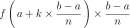
ELi [f(a + kx b -^ on the integral. If, for examp
n
the integral f b f(t) dt ‘inherits’ the dimension of the approximating sum
The notation f% f(t) dt helps keep track of the units of dimension e, f(t) is the velocity of a particle, the factor (b — a)/n in the approximating sum will have units of time, f(a + k x ^) x (b — a)/n will have units of distance, and the approximating sum and the integral will have units of distance. In f(t) dt, f(t) has units of velocity, dt can be considered to have units of time so that f(t) dt has units of distance and fa /(0 dt nas un its of distance.
Example 9.4.1 The answers to examples and exercises of sections 9.1 through 9.3 all may be expressed in terms of integrals:
I. The area of the region bounded by the graphs of y — f(t) > 0, y = 0, t = a and t = b is
la f(t) ^.
2. The mass of a body of density D(x) and cross sectional area A(x) along an interval [a, b] is f b a D(x) x A(x) dx.
5 A good source of this debate is in Philip J. Davis and Reuben Hersh, The Mathematical Experience, Houghton Mifflin Co., Boston, 1982.
CHAPTER 9. THE INTEGRAL
433
3. The work done by the heart during one heart beat is J 6 e R(t) x P(t) dt where R is aortic flow rate and P is pressure in the left ventricle. The units on this integral are
ml cm 3 N
R(t) — x 1 —- x Pit) — ft x dt sec = N-cm sec ml cm
which is a unit of work. Had the units not been of work, we would think that the integral is incorrectly formulated.
4. Atmospheric density at altitude h meters is approximately 1.225e~ 0 000101h kg/m 3 for
0 < a < 5000. The mass of air in a one square meter vertical column between 1000 and 4000 meters is J$°° 1.225e-° 000101/l xldh. m
Example 9.4.2 We use Definition 9.4.1 to compute the area of the region R bounded by
y = x 2 (2 — x) = 2x 2 — x 3 , y = 0, x = 0, and x = 2. The region for which we wish to compute the
area is shown in Figure 9.4.2.2 and the area is
1-2
2x 2 — x 3 dx
Figure for Example 9.4.2.2 The region R bounded by y = x 2 (2 — x) and y = 0.
Following Equation 9.14, partition [0,2] into n subintervals 0, 2/n, 2(2/n), 3(2/n) ■ ■ ■ n(2/n) = 2 each of length 2/n. Then write the sum
r2 n
f – ( k(2/n) f) x 2/n
J 2x 2 -x 3 dx = hm £j (2 ( k(2/n)
2 um (y k 2 ) ^ – hm (y k 3 ) –
™ Vjfcl / n 3 n^oo J n
2 hm n(n + l)(2n + l)23 _
6
n’
n 2 (n+ 1) 2 2 4
n
CHAPTER 9. THE INTEGRAL
434
The area of R is 4/3. We computed an approximation of 1.32 to this area in Example 9.2.2. i
Example 9.4.3 We use Definition 9.4.1 to compute the area of the region bounded by y = e*, y = 0, t = 0, and t = x. The region for which we wish to compute the area is shown in Figure 9.4.3.3 and we wish to compute
/ e* dt. Jo
Equation 9.14 evaluates the integrand at the right end of each interval, and for this particular problem it is slightly simpler to evaluate the integrand at the left end points and compute
lim
n—too
J2f [a + (k-l)x
L k=l \
n
b — a
n
The effect is to change from an upper approximation to a lower approximation. Figure for Example 9.4.3.3 The region bounded by y — e*, y — 0, t — 0 and t = x.
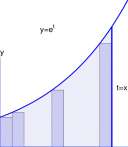
(k-i)h
We recall a formula for the sum of a geometric series:
a n — 1
l+a + a 2 + a z + —+a n ~ l = (9.15)
a — 1
This formula can be confirmed by multiplication of
(1 – a) x (l + a + a 2 + a 3 H h a 71 ” 1 )
Assume the interval [0,x] to be partitioned into n equal subintervals, each of length x/n and we let h = x/n. The k th such interval has endpoints on the t axis at (k — 1) x h and k x h. The area of the fc th rectangle is
e (k-l)x(x/n) x ^ = e ( k -l)x(h) x ^
n
and the sum of the areas of the n rectangles is
n
J2 e {k ~ l)xh x h k=i
CHAPTER 9. THE INTEGRAL
435
Our job is to make sense of
y e {k 1)xh x fc because [* e* dt = lim V e (fc 1)x/l x fc.
k=l JU fc=l
Observe that so that
0 (k-l)xh x
fc=(e>)
X fc
£ e (fc-l)xh x h k=l
EM
fc-i
k=\
x fc.
We write the part in [ ]’s in long format with a generic term as k = 1 fc = 2 fc
k = n
n-l
(e h )° + (e 71 ) 1 + ••• +(e h ) k 1 + ••• + (e n With a = e h the preceding sum is the geometric series shown in Equation 9.15 and we conclude that
x fc
k=l
e h – 1
= (e*-l)xA
Now the problem is to evaluate
f e* d* = lim V e (fc 1)xW x fc = lim ( e x -l)x^— = (e x – 1) x \
J 0 n->oo ^ n-t-oo V ‘ e h -l V / e — 1
lim
h^O h
By its definition, Definition 5.2.1 on page 219, the number e has the property that
We conclude that
lim — = 1.
h^O h
e* dt = e x – 1
Example 9.4.4 Use the trigonometric identity Bolt out of the Blue! 6
sm/c6*
fc=i
— cos{nu + -) + cos –
2 sin
0
and lim
sin(fc)
h^O h
6 The Blue: Use 2 sin x sin y = — cos(a; + y) + cos(x — y). Let S = J2k=i s ^ n kd. Then
9 ™ 6 n
25 sin – = 2 y sin fc0 sin – = ^ (- cos(fc(9 + 6/2) + cos(fc<9 – 0/2))
k=l k=l
(- cos(0 + 6>/2) + cos(6> – 0/2)) + (- cos(20 + 6/2) + cos(20 – 6/2)) + ••• + (- cos(n0 + 6/2) + cos(n0 – 6/2)) (- cos(30/2) + cos(0/2)) + (- cos(50/2) + cos(30/2)) + ••• + (- cos(n0 + 6/2) + cos(n0 – 6/2))
= – cos(nd + 6/2) + cos(0/2)
CHAPTER 9. THE INTEGRAL
436
to compute Jq sint dt, for 0 < x < ir. The integral is the area of a segment, R, of the sine curve shown in Figure 9.4.4.4.
Figure for Example 9.4.4.4 The region, R, bounded by y = sint and y = 0 between t = 0 and
t = x, and a typical fcth rectangle.
Partition the interval [0,x] into n equal subintervals by tk = k x x/n. Then
/ sin t dt = lim (sin it) x (tu — tu-i) J * ™ fx
lim (sin(/c X —)) x —
n ^°° ^ V n ) n
– cosfn x – + —) + cost—) „ lim x *
2 sin— n 2n
x x \ —
lim ( — cos(x + —) +cos(—) ) . 2 “_ 2n 2n ) sin
In
X
lim (— cosfa; H )) + lim cos(—)) lim —— r
n-^oo ATI n^oo ATI J n ^°° •
sin —
2n
COS X + COS 0) X 1 = 1 — COS X
Specifically,
7r/2 Tj- /-7T
sin t dt = 1 — cos — = 1, and / sini dt = 1 — cos7r = 2. ■ o 2 ‘ 7o
9.4.1 A more flexible definition of integral.
The sum in Definition of Integral I 9.4.1 uses intervals of equal length and evaluates / at the right end point of each interval. In order to provide some flexibility in computation of approximating sums (upper, lower or any of the others) and variable interval sizes, the following definitions are used.
Definition 9.4.2 Partition of an interval. Suppose [a, b] is an interval. A partition of [a, b] is a sequence, A, of numbers
a — t 0 < h < t 2 • • • < t k • • • < t n -i <t n = b
The norm of the partition, denoted by ||A||, is the largest length of any interval between successive members of A.
||A|| = Max{ti – t 0 ,t 2 — h,—t k — t k -i ■■■t n – t n _i}
Definition 9.4.3 Approximating sum to an integral. Suppose / is a function defined on an interval [a, b] . An approximating sum for the integral of / on [a, b] is a number of the form
/(n) x (*! – t 0 ) + /(r 2 ) x (t 2 – h) + ■ ■ ■ + fin) x (t k – tfc_i) + • • • + f(r n ) x (t n – t n -i)
where a = t 0 < t\ < t 2 ■ • ■ < £ n -i < t n — b is a partition of [a, b] and
to<n<t 1 t 1 <r 2 <t 2 ■■■ t k _ 1 <r k <t k ■■■ t n _ 1 <T n <t n
Definition 9.4.4 The integral of a function, II. Suppose / is an increasing function defined on an interval [a, b]. The integral of / on [a, b] is denoted by J a b fit) dt and defined by
[ b f(t)dt=\im J2 f( T «) x (** – **-0 ( 9 16 )
Ja ||A|H0 fc=1
Implicit in the previous symbol is that A = a = t 0 < t\ < t 2 • • • < t k ■ ■ • < t n -i < tn — b is a partition of [a, b] and that t k -i < i~ k <t k for k — l,n.
The two definitions of integral give a unique number and the same number for all increasing functions and for all decreasing functions and for all functions that alternate between increasing and decreasing only a finite number of times on [a, b]. Definition I is easier to comprehend, but the flexibility in Definition II in computing the approximating sum is sometimes helpful.
There are some functions for which either the limits in Definitions I and II are different or do not exist. It is unlikely that you will encounter one in undergraduate study, and we will not discuss them. We will assume that for all functions we deal with, the limits in Definitions I and II exist and are the same. For such functions, we say the the integral exists and we say the functions are integrable.
Exercises for Section 9.4, The Integral.
Exercise 9.4.1 a. The area formulas shown in Exercise Figure 9.4.1 were shown to be valid in Section 9.2 and are summarized in Equations 9.8 found in Exercise 9.2.12. Write these area formulas as integral formulas. One of them, for example, will be