5.E: Integration (Exercises)

These are homework exercises to accompany OpenStax's "Calculus" Textmap.

5.1: Approximating Areas

1.) State whether the given sums are equal or unequal.

1. \(\displaystyle \sum_{i=1}^{10}i\) and \(\displaystyle \sum_{k=1}^{10}k\)
2. \(\displaystyle \sum_{i=1}^{10}i\) and \(\displaystyle \sum_{i=6}^{15}(i−5)\)
3. \(\displaystyle \sum_{i=1}^{10}i(i−1)\) and \(\displaystyle \sum_{j=0}^9(j+1)j\)
4. \(\displaystyle \sum_{i=1}^{10}i(i−1)\) and \(\displaystyle \sum_{k=1}^{10}(k^2−k)\)

Solution: a. They are equal; both represent the sum of the first 10 whole numbers. b. They are equal; both represent the sum of the first 10 whole numbers. c. They are equal by substituting \(\displaystyle j=i−1.\) d. They are equal; the first sum factors the terms of the second.

In the following exercises, use the rules for sums of powers of integers to compute the sums.

2) \(\displaystyle \sum_{i=5}^{10}i\)

3) \(\displaystyle \sum_{i=5}^{10}i^2\)

Solution: \(\displaystyle 385−30=355\)

Suppose that \(\displaystyle \sum_{i=1}^{100}a_i=15\) and \(\displaystyle \sum_{i=1}^{100}b_i=−12.\) In the following exercises, compute the sums.

4) \(\displaystyle \sum_{i=1}^{100}(a_i+b_i)\)

5) \(\displaystyle \sum_{i=1}^{100}(a_i−b_i)\)

Solution: \(\displaystyle 15−(−12)=27\)

6) \(\displaystyle \sum_{i=1}^{100}(3a_i−4b_i)\)

7) \(\displaystyle \sum_{i=1}^{100}(5a_i+4b_i)\)

Solution: \(\displaystyle 5(15)+4(−12)=27\)

In the following exercises, use summation properties and formulas to rewrite and evaluate the sums.

8) \(\displaystyle \sum_{k=1}^{20}100(k^2−5k+1)\)

9) \(\displaystyle \sum_{j=1}^{50}(j^2−2j)\)

Solution: \(\displaystyle \sum_{j=1}^{50}j%2−2\sum_{j=1}^{50}j=\frac{(50)(51)(101)}{6}−\frac{2(50)(51)}{2}=40, 375\)

10) \(\displaystyle \sum_{j=11}^{20}(j^2−10j)\)

11) \(\displaystyle \sum_{k=1}^{25}[(2k)^2−100k]\)

Solution: \(\displaystyle 4\sum_{k=1}^{25}k^2−100\sum_{k=1}^{25}k=\frac{4(25)(26)(51)}{9}−50(25)(26)=−10, 400\)

Let \(\displaystyle L_n\) denote the left-endpoint sum using n subintervals and let \(\displaystyle R_n\) denote the corresponding right-endpoint sum. In the following exercises, compute the indicated left and right sums for the given functions on the indicated interval.

12) \(\displaystyle L_4\) for \(\displaystyle f(x)=\frac{1}{x−1}\) on \(\displaystyle [2,3]\)

13) \(\displaystyle R_4\) for \(\displaystyle g(x)=cos(πx)\) on \(\displaystyle [0,1]\)

Solution: \(\displaystyle R_4=0.25\)

14) \(\displaystyle L_6\) for \(\displaystyle f(x)=\frac{1}{x(x−1)}\) on \(\displaystyle [2,5]\)

15) \(\displaystyle R_6\) for \(\displaystyle f(x)=\frac{1}{x(x−1)}\) on \(\displaystyle [2,5]\)

Solution: \(\displaystyle R_6=0.372\)

16) \(\displaystyle R_4\) for \(\displaystyle \frac{1}{x^2+1}\) on \(\displaystyle [−2,2]\)

17) \(\displaystyle L_4\) for \(\displaystyle \frac{1}{x^2+1}\) on \(\displaystyle [−2,2]\)

\(\displaystyle L_4=2.20\)

18) \(\displaystyle R_4\) for \(\displaystyle x^2−2x+1\) on \(\displaystyle [0,2]\)

19) \(\displaystyle L_8\) for \(\displaystyle x^2−2x+1\) on \(\displaystyle [0,2]\)

Solution: \(\displaystyle L_8=0.6875\)

20) Compute the left and right Riemann sums— \(\displaystyle L_4\) and \(\displaystyle R_4\), respectively—for \(\displaystyle f(x)=(2−|x|)\) on \(\displaystyle [−2,2].\) Compute their average value and compare it with the area under the graph of f.

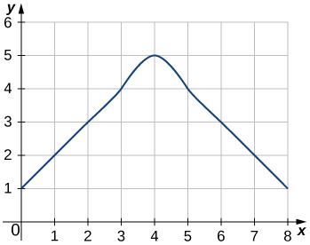
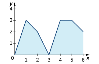
21) Compute the left and right Riemann sums— \(\displaystyle L_6\) and \(\displaystyle R_6\), respectively—for \(\displaystyle f(x)=(3−|3−x|)\) on \(\displaystyle [0,6].\) Compute their average value and compare it with the area under the graph of f.

Solution: \(\displaystyle L_6=9.000=R_6\). The graph of f is a triangle with area 9.

22) Compute the left and right Riemann sums— \(\displaystyle L_4\) and \(\displaystyle R_4\), respectively—for \(\displaystyle f(x)=\sqrt{4−x^2}\) on \(\displaystyle [−2,2]\) and compare their values.

23) Compute the left and right Riemann sums— \(\displaystyle L_6\) and \(\displaystyle R_6\), respectively—for \(\displaystyle f(x)=\sqrt{9−(x−3)^2}\) on \(\displaystyle [0,6]\) and compare their values.

Solution: \(\displaystyle L_6=13.12899=R_6\). They are equal.

Express the following endpoint sums in sigma notation but do not evaluate them.

24) \(\displaystyle L_{30}\) for \(\displaystyle f(x)=x^2\) on \(\displaystyle [1,2]\)

25) \(\displaystyle L_{10}\) for \(\displaystyle f(x)=\sqrt{4−x^2}\) on \(\displaystyle [−2,2]\)

Solution: \(\displaystyle L_{10}=\frac{4}{10}\sum_{i=1}^{10}\sqrt{4−(−2+4\frac{(i−1)}{10})}\)

26) \(\displaystyle R_{20}\) for \(\displaystyle f(x)=sinx\) on \(\displaystyle [0,π]\)

27) \(\displaystyle R_{100}\) for \(\displaystyle lnx\) on \(\displaystyle [1,e]\)

Solution: \(\displaystyle R_{100}=\frac{e−1}{100}\sum_{i=1}^{100}ln(1+(e−1)\frac{i}{100})\)

In the following exercises, graph the function then use a calculator or a computer program to evaluate the following left and right endpoint sums. Is the area under the curve between the left and right endpoint sums?

28) [T] \(\displaystyle L_{100}\) and \(\displaystyle R_{100}\) for \(\displaystyle y=x^2−3x+1\) on the interval \(\displaystyle [−1,1]\)

29) [T] \(\displaystyle L_{100}\) and \(\displaystyle R_{100}\) for \(\displaystyle y=x^2\) on the interval \(\displaystyle [0,1]\)

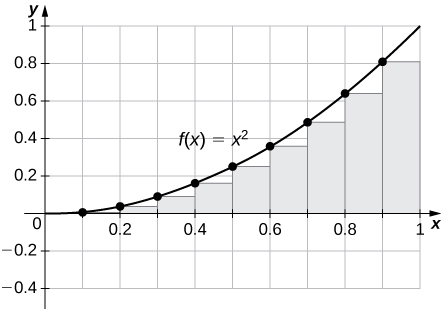
\(\displaystyle R_{100}=0.33835,L_{100}=0.32835.\) The plot shows that the left Riemann sum is an underestimate because the function is increasing. Similarly, the right Riemann sum is an overestimate. The area lies between the left and right Riemann sums. Ten rectangles are shown for visual clarity. This behavior persists for more rectangles.

30) [T] \(\displaystyle L_{50}\) and \(\displaystyle R_{50}\) for \(\displaystyle y=\frac{x+1}{x^2−1}\) on the interval \(\displaystyle [2,4]\)

31) [T] \(\displaystyle L_{100}\) and \(\displaystyle R_{100}\) for \(\displaystyle y=x^3\) on the interval \(\displaystyle [−1,1]\)

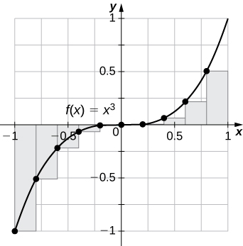
\(\displaystyle L_{100}=−0.02,R_{100}=0.02\). The left endpoint sum is an underestimate because the function is increasing. Similarly, a right endpoint approximation is an overestimate. The area lies between the left and right endpoint estimates.

32) [T] \(\displaystyle L_{50}\) and \(\displaystyle R_{50}\) for \(\displaystyle y=tan(x)\) on the interval \(\displaystyle [0,\frac{π}{4}]\)

33) [T] \(\displaystyle L_{100}\) and \(\displaystyle R_{100}\) for \(\displaystyle y=e^{2x}\) on the interval \(\displaystyle [−1,1]\)

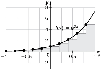
\(\displaystyle L_{100}=3.555,R_{100}=3.670\). The plot shows that the left Riemann sum is an underestimate because the function is increasing. Ten rectangles are shown for visual clarity. This behavior persists for more rectangles.

34) Let \(\displaystyle t_j\) denote the time that it took Tejay van Garteren to ride the jth stage of the Tour de France in 2014. If there were a total of 21 stages, interpret \(\displaystyle \sum_{j=1}^{21}t_j\).

35) Let \(\displaystyle r_j\) denote the total rainfall in Portland on the jth day of the year in 2009. Interpret \(\displaystyle \sum_{j=1}^{31}r_j\).

Solution: The sum represents the cumulative rainfall in January 2009.

36) Let \(\displaystyle d_j\) denote the hours of daylight and \(\displaystyle δ_j\) denote the increase in the hours of daylight from day \(\displaystyle j−1\) to day j in Fargo, North Dakota, on thejth day of the year. Interpret \(\displaystyle d1+\sum_{j=2}^{365}δ_j\).

37) To help get in shape, Joe gets a new pair of running shoes. If Joe runs 1 mi each day in week 1 and adds \(\displaystyle \frac{1}{10}\) mi to his daily routine each week, what is the total mileage on Joe’s shoes after 25 weeks?

Solution: The total mileage is \(\displaystyle 7×\sum_{i=1}^{25}(1+\frac{(i−1)}{10})=7×25+\frac{7}{10}×12×25=385mi\).

38) The following table gives approximate values of the average annual atmospheric rate of increase in carbon dioxide (CO₂) each decade since 1960, in parts per million (ppm). Estimate the total increase in atmospheric CO₂ between 1964 and 2013.

Decade	Ppm/y
1964-1973	1.07
1976-1983	1.34
1984-1993	1.40
1994-2003	1.87
2004-2013	2.07

Average Annual Atmospheric CO2 Increase, 1964–2013 Source: http://www.esrl.noaa.gov/gmd/ccgg/trends/.

39) The following table gives the approximate increase in sea level in inches over 20 years starting in the given year. Estimate the net change in mean sea level from 1870 to 2010.

Starting Year	20- Year Change
1870	0.3
1890	1.5
1910	0.2
1930	2.8
1950	0.7
1970	1.1
1990	1.5

Approximate 20-Year Sea Level Increases, 1870–1990

Source: http://link.springer.com/article/10....712-011-9119-1

Solution: Add the numbers to get 8.1-in. net increase.

40) The following table gives the approximate increase in dollars in the average price of a gallon of gas per decade since 1950. If the average price of a gallon of gas in 2010 was $2.60, what was the average price of a gallon of gas in 1950?

Starting Year	10- Year Change
1950	0.03
1960	0.05
1970	0.86
1980	−0.03
1990	0.29
2000	1.12

Approximate 10-Year Gas Price Increases, 1950–2000

Source: http://epb.lbl.gov/homepages/Rick_Di...011-trends.pdf.

41) The following table gives the percent growth of the U.S. population beginning in July of the year indicated. If the U.S. population was 281,421,906 in July 2000, estimate the U.S. population in July 2010.

Year	% Change/Year
2000	1.12
2001	0.99
2002	0.93
2003	0.86
2004	0.93
2005	0.93
2006	0.97
2007	0.96
2008	0.95
2009	0.88

Annual Percentage Growth of U.S. Population, 2000–2009

Source: http://www.census.gov/popest/data.

(Hint: To obtain the population in July 2001, multiply the population in July 2000 by 1.0112 to get 284,573,831.)

Solution: 309,389,957

In the following exercises, estimate the areas under the curves by computing the left Riemann sums, \(\displaystyle L_8.\)

42)

43)

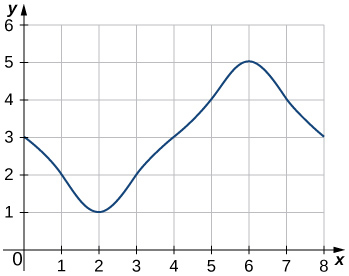
Solution: \(\displaystyle L_8=3+2+1+2+3+4+5+4=24\)

44)

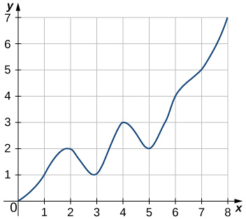
45)

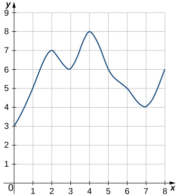
Solution: \(\displaystyle L_8=3+5+7+6+8+6+5+4=44\)

46) [T] Use a computer algebra system to compute the Riemann sum, \(\displaystyle L_N\), for \(\displaystyle N=10,30,50\) for \(\displaystyle f(x)=\sqrt{1−x^2}\) on \(\displaystyle [−1,1].\)

47) [T] Use a computer algebra system to compute the Riemann sum, \(\displaystyle L_N\), for \(\displaystyle N=10,30,50\) for \(\displaystyle f(x)=\frac{1}{\sqrt{1+x^2}}\) on \(\displaystyle [−1,1].\)

Solution: \(\displaystyle L_{10}≈1.7604,L_{30}≈1.7625,L_{50}≈1.76265\)

48) [T] Use a computer algebra system to compute the Riemann sum, \(\displaystyle L_N\), for \(\displaystyle N=10,30,50\) for \(\displaystyle f(x)=sin^2x\) on \(\displaystyle [0,2π]\). Compare these estimates with π.

In the following exercises, use a calculator or a computer program to evaluate the endpoint sums \(\displaystyle R_N\) and \(\displaystyle L_N\) for \(\displaystyle N=1,10,100\). How do these estimates compare with the exact answers, which you can find via geometry?

49) [T] \(\displaystyle y=cos(πx)\) on the interval \(\displaystyle [0,1]\)

Solution: \(\displaystyle R_1=−1,L_1=1,R_{10}=−0.1,L_{10}=0.1,L_{100}=0.01,\) and \(\displaystyle R_{100}=−0.1.\) By symmetry of the graph, the exact area is zero.

50) [T] \(\displaystyle y=3x+2\) on the interval \(\displaystyle [3,5]\)

In the following exercises, use a calculator or a computer program to evaluate the endpoint sums \(\displaystyle R_N\) and \(\displaystyle L_N\) for \(\displaystyle N=1,10,100.\)

51) [T] \(\displaystyle y=x^4−5x^2+4\) on the interval \(\displaystyle [−2,2]\), which has an exact area of \(\displaystyle \frac{32}{15}\)

Solution: \(\displaystyle R_1=0,L_1=0,R_{10}=2.4499,L_{10}=2.4499,R_{100}=2.1365,L_{100}=2.1365\)

52) [T] \(\displaystyle y=lnx\) on the interval \(\displaystyle [1,2]\), which has an exact area of \(\displaystyle 2ln(2)−1\)

53) Explain why, if \(\displaystyle f(a)≥0\) and f is increasing on \(\displaystyle [a,b]\), that the left endpoint estimate is a lower bound for the area below the graph of \(\displaystyle f\) on \(\displaystyle [a,b].\)

Solution: If \(\displaystyle [c,d]\)is a subinterval of \(\displaystyle [a,b]\) under one of the left-endpoint sum rectangles, then the area of the rectangle contributing to the left-endpoint estimate is \(\displaystyle f(c)(d−c)\). But, \(\displaystyle f(c)≤f(x)\) for \(\displaystyle c≤x≤d\), so the area under the graph of \(\displaystyle f\) between \(\displaystyle c\) and \(\displaystyle d\) is \(\displaystyle f(c)(d−c)\) plus the area below the graph of f but above the horizontal line segment at height \(\displaystyle f(c)\), which is positive. As this is true for each left-endpoint sum interval, it follows that the left Riemann sum is less than or equal to the area below the graph of \(\displaystyle f\) on \(\displaystyle [a,b].\)

54) Explain why, if \(\displaystyle f(b)≥0\) and f is decreasing on \(\displaystyle [a,b],\) that the left endpoint estimate is an upper bound for the area below the graph of \(\displaystyle f\) on \(\displaystyle [a,b].\)

55) Show that, in general, \(\displaystyle R_N−L_N=(b−a)×\frac{f(b)−f(a)}{N}.\)

Solution: \(\displaystyle L_N=\frac{b−a}{N}\sum_{i=1}^Nf(a+(b−a)\frac{i−1}{N})=\frac{b−a}{N}\sum_{i=0}^{N−1}f(a+(b−a)\frac{i}{N})\) and \(\displaystyle R_N=\frac{b−a}{N}\sum_{i=1}^Nf(a+(b−a)\frac{i}{N})\). The left sum has a term corresponding to \(\displaystyle i=0\) and the right sum has a term corresponding to \(\displaystyle i=N\). In \(\displaystyle R_N−L_N\), any term corresponding to \(\displaystyle i=1,2,…,N−1\) occurs once with a plus sign and once with a minus sign, so each such term cancels and one is left with \(\displaystyle R_N−L_N=\frac{b−a}{N}(f(a+(b−a))\frac{N}{N})−(f(a)+(b−a)\frac{0}{N})=\frac{b−a}{N}(f(b)−f(a)).\)

56) Explain why, if f is increasing on [ \(\displaystyle a,b\)], the error between either \(\displaystyle L_N\) or \(\displaystyle R_N\) and the area A below the graph of f is at most \(\displaystyle (b−a)\frac{f(b)−f(a)}{N]|).

57) For each of the three graphs:

a. Obtain a lower bound \(\displaystyle L(A)\) for the area enclosed by the curve by adding the areas of the squares enclosed completely by the curve.

b. Obtain an upper bound \(\displaystyle U(A)\) for the area by adding to \(\displaystyle L(A)\) the areas \(\displaystyle B(A)\) of the squares enclosed partially by the curve.

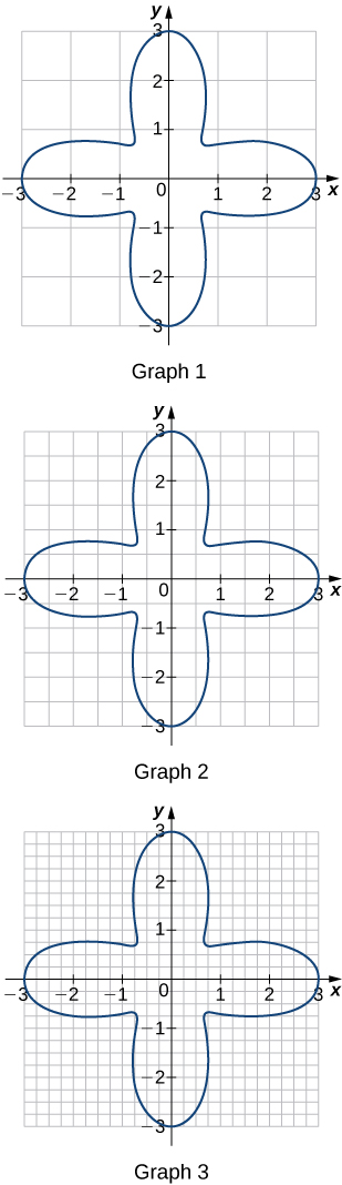
Solution: Graph 1: a. \(\displaystyle L(A)=0,B(A)=20; b. U(A)=20.\) Graph 2: \(\displaystyle a. L(A)=9; b. B(A)=11,U(A)=20.\) Graph 3: a. \(\displaystyle L(A)=11.0; b. B(A)=4.5,U(A)=15.5.\)

58) In the previous exercise, explain why \(\displaystyle L(A)\) gets no smaller while \(\displaystyle U(A)\) gets no larger as the squares are subdivided into four boxes of equal area.

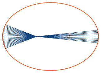
59) A unit circle is made up of n wedges equivalent to the inner wedge in the figure. The base of the inner triangle is 1 unit and its height is \(\displaystyle sin(\frac{π}{n}).\) The base of the outer triangle is \(\displaystyle B=cos(\frac{π}{n})+sin(\frac{π}{n})tan(\frac{π}{n})\) and the height is \(\displaystyle H=Bsin(\frac{2π}{n})\). Use this information to argue that the area of a unit circle is equal to π.\)

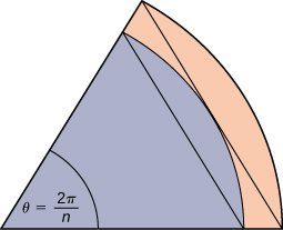
Let A be the area of the unit circle. The circle encloses n congruent triangles each of area \(\displaystyle \frac{sin(\frac{2π}{n})}{2}\), so \(\displaystyle \frac{n}{2}sin(\frac{2π}{n})≤A.\) Similarly, the circle is contained inside n congruent triangles each of area \(\displaystyle \frac{BH}{2}=\frac{1}{2}(cos(\frac{π}{n})+sin(\frac{π}{n})tan(\frac{π}{n}))sin(\frac{2π}{n})\), so \(\displaystyle A≤\frac{n}{2}sin(\frac{2π}{n})(cos(\frac{π}{n}))+sin(\frac{π}{n})tan(\frac{π}{n})\). As \(\displaystyle n→∞,\frac{n}{2}sin(\frac{2π}{n})=\frac{πsin(\frac{2π}{n})}{(\frac{2π}{n})}→π\), so we conclude \(\displaystyle π≤A\). Also, as \(\displaystyle n→∞,cos(\frac{π}{n})+sin(\frac{π}{n})tan(\frac{π}{n})→1\), so we also have \(\displaystyle A≤π\). By the squeeze theorem for limits, we conclude that \(\displaystyle A=π.\)

5.2: The Definite Integral

In the following exercises, express the limits as integrals.

1) \(\displaystyle \lim_{n→∞}\sum_{i=1}^n(x^∗_i)Δx\) over \(\displaystyle [1,3]\)

2) \(\displaystyle \lim_{n→∞}\sum_{i=1}^n(5(x^∗_i)^2−3(x^∗_i)^3)Δx\) over \(\displaystyle [0,2]\)

Solution: \(\displaystyle ∫^2_0(5x^2−3x^3)dx\)

3) \(\displaystyle \lim_{n→∞}\sum_{i=1}^nsin^2(2πx^∗_i)Δx\) over \(\displaystyle [0,1]\)

4) \(\displaystyle \lim_{n→∞}\sum_{i=1}^ncos^2(2πx^∗_i)Δx\) over \(\displaystyle [0,1]\)

Solution: \(\displaystyle ∫^1_0cos^2(2πx)dx\)

In the following exercises, given \(\displaystyle L_n\) or \(\displaystyle R_n\) as indicated, express their limits as \(\displaystyle n→∞\) as definite integrals, identifying the correct intervals.

5) \(\displaystyle L_n=\frac{1}{n}\sum_{i=1}^n\frac{i−1}{n}\)

6) \(\displaystyle R_n=\frac{1}{n}\sum_{i=1}^n\frac{i}{n}\)

Solution: \(\displaystyle ∫^1_0xdx\)

7) \(\displaystyle Ln=\frac{2}{n}\sum_{i=1}^n(1+2\frac{i−1}{n})\)

8) \(\displaystyle R_n=\frac{3}{n}\sum_{i=1}^n(3+3\frac{i}{n})\)

Solution: \(\displaystyle ∫^6_3xdx\)

9) \(\displaystyle L_n=\frac{2π}{n}\sum_{i=1}^n2π\frac{i−1}{n}cos(2π\frac{i−1}{n})\)

10 \(\displaystyle R_n=\frac{1}{n}\sum_{i=1}^n(1+\frac{i}{n})log((1+\frac{i}{n})^2)\)

Solution: \(\displaystyle ∫^2_1xlog(x^2)dx\)

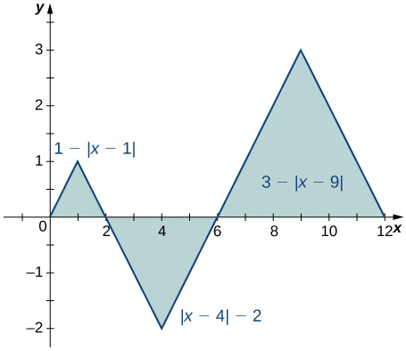
In the following exercises, evaluate the integrals of the functions graphed using the formulas for areas of triangles and circles, and subtracting the areas below the x-axis.

11)

12)

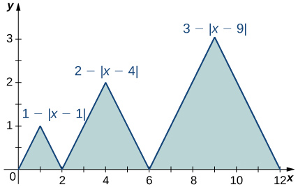
Solution: \(\displaystyle 1+2⋅2+3⋅3=14\)

13)

14)

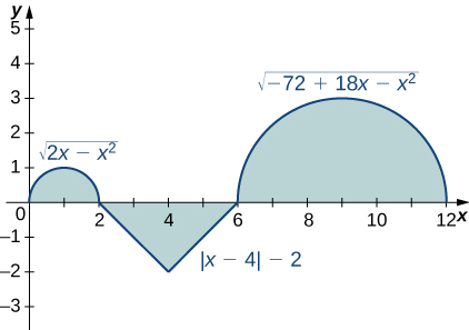
Solution: \(\displaystyle 1−4+9=6\)

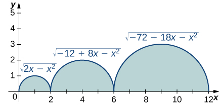
15)

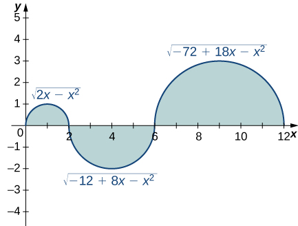
16)

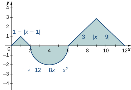
Solution: \(\displaystyle 1−2π+9=10−2π\)

In the following exercises, evaluate the integral using area formulas.

17) \(\displaystyle ∫^3_0(3−x)dx\)

18) \(\displaystyle ∫^3_2(3−x)dx\)

Solution: The integral is the area of the triangle, \(\displaystyle \dfrac{1}{2}\)

19) \(\displaystyle ∫^3_{−3}(3−|x|)dx\)

20) \(\displaystyle ∫^6_0(3−|x−3|)dx\)

Solution: The integral is the area of the triangle, \(\displaystyle 9.\)

21) \(\displaystyle ∫^2_{−2}\sqrt{4−x^2}dx\)

22) \(\displaystyle ∫^5_1\sqrt{4−(x−3)^2}dx\)

Soluti0n: The integral is the area \(\displaystyle \frac{1}{2}πr^2=2π.\)

23) \(\displaystyle ∫^{12}_0\sqrt{36−(x−6)^2}dx\)

24) \(\displaystyle ∫^3_{−2}(3−|x|)dx\)

Solution: The integral is the area of the “big” triangle less the “missing” triangle, \(\displaystyle 9−\frac{1}{2}.\)

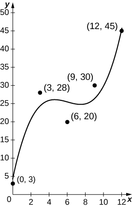
In the following exercises, use averages of values at the left (L) and right (R) endpoints to compute the integrals of the piecewise linear functions with graphs that pass through the given list of points over the indicated intervals.

25) \(\displaystyle {(0,0),(2,1),(4,3),(5,0),(6,0),(8,3)}\) over \(\displaystyle [0,8]\)

26) \(\displaystyle {(0,2),(1,0),(3,5),(5,5),(6,2),(8,0)}\) over \(\displaystyle [0,8]\)

Solution: \(\displaystyle L=2+0+10+5+4=21,R=0+10+10+2+0=22,\dfrac{L+R}{2}=21.5\)

27) \(\displaystyle {(−4,−4),(−2,0),(0,−2),(3,3),(4,3)}\) over \(\displaystyle [−4,4]\)

28) \(\displaystyle {(−4,0),(−2,2),(0,0),(1,2),(3,2),(4,0)}\) over \(\displaystyle [−4,4]\)

Solution: \(\displaystyle L=0+4+0+4+2=10,R=4+0+2+4+0=10,\dfrac{L+R}{2}=10\)

Suppose that \(\displaystyle ∫^4_0f(x)dx=5\) and \(\displaystyle ∫^2_0f(x)dx=−3\), and \(\displaystyle ∫^4_0g(x)dx=−1\) and \(\displaystyle ∫^2_0g(x)dx=2\). In the following exercises, compute the integrals.

29) \(\displaystyle ∫^4_0(f(x)+g(x))dx\)

30) \(\displaystyle ∫^4_2(f(x)+g(x))dx\)

Solution: \(\displaystyle ∫^4_2f(x)dx+∫^4_2g(x)dx=8−3=5\)

31) \(\displaystyle ∫^2_0(f(x)−g(x))dx\)

32) \(\displaystyle ∫^4_2(f(x)−g(x))dx\)

Solution: \(\displaystyle ∫^4_2f(x)dx−∫^4_2g(x)dx=8+3=11\)

33) \(\displaystyle ∫^2_0(3f(x)−4g(x))dx\)

34) \(\displaystyle ∫^4_2(4f(x)−3g(x))dx\)

Solution: \(\displaystyle 4∫^4_2f(x)dx−3∫^4_2g(x)dx=32+9=41\)

In the following exercises, use the identity \(\displaystyle ∫^A_{−A}f(x)dx=∫^0_{−A}f(x)dx+∫^A_0f(x)dx\) to compute the integrals.

35) \(\displaystyle ∫^π_{−π}\frac{sint}{1+t^2}dt\) (Hint: \(\displaystyle sin(−t)=−sin(t))\)

36) \(\displaystyle ∫^{\sqrt{π}}_\sqrt{−π}\frac{t}{1+cost}dt\)

Solution: The integrand is odd; the integral is zero.

37) \(\displaystyle ∫^3_1(2−x)dx\) (Hint: Look at the graph of f.)

38) \(\displaystyle ∫^4_2(x−3)^3dx\) (Hint: Look at the graph of f.)

Solution: The integrand is antisymmetric with respect to \(\displaystyle x=3.\) The integral is zero.

In the following exercises, given that \(\displaystyle ∫^1_0xdx=\frac{1}{2},∫^1_0x^2dx=\frac{1}{3},\) and \(\displaystyle ∫^1_0x^3dx=\frac{1}{4}\), compute the integrals.

39) \(\displaystyle ∫^1_0(1+x+x^2+x^3)dx\)

40) \(\displaystyle ∫^1_0(1−x+x^2−x^3)dx\)

Solution: \(\displaystyle 1−\frac{1}{2}+\frac{1}{3}−\frac{1}{4}=\frac{7}{12}\)

41) \(\displaystyle ∫^1_0(1−x)^2dx\)

42) \(\displaystyle ∫^1_0(1−2x)^3dx\)

Solution: \(\displaystyle ∫^1_0(1−2x+4x^2−8x^3)dx=1−1+\frac{4}{3}−2=−\frac{2}{3}\)

43) \(\displaystyle ∫^1_0(6x−\frac{4}{3}x^2)dx\)

44) \(\displaystyle ∫^1_0(7−5x^3)dx\)

Solution: \(\displaystyle 7−\frac{5}{4}=\frac{23}{4}\)

In the following exercises, use the comparison theorem.

45) Show that \(\displaystyle ∫^3_0(x^2−6x+9)dx≥0.\)

46) Show that \(\displaystyle ∫^3_{−2}(x−3)(x+2)dx≤0.\)

Solution: The integrand is negative over \(\displaystyle [−2,3].\)

47) Show that \(\displaystyle ∫^1_0\sqrt{1+x^3}dx≤∫^1_0\sqrt{1+x^2}dx\).

48) Show that \(\displaystyle ∫^2_1\sqrt{1+x}dx≤∫^2_1\sqrt{1+x^2}dx.\)

Solution: \(\displaystyle x≤x^2\) over \(\displaystyle [1,2]\), so \(\displaystyle \sqrt{1+x}≤\sqrt{1+x^2}\) over \(\displaystyle [1,2].\)

49) Show that \(\displaystyle ∫^{π/2}_0sintdt≥\frac{π}{4})\) (Hint: \(\displaystyle sint≥\frac{2t}{π}\) over \(\displaystyle [0,\frac{π}{2}])\)

50) Show that \(\displaystyle ∫^{π/4}_{−π/4}costdt≥π\sqrt{2}/4\).

Solution: \(\displaystyle cos(t)≥\dfrac{\sqrt{2}}{2}\). Multiply by the length of the interval to get the inequality.

In the following exercises, find the average value \(\displaystyle f_{ave}\) of f between a and b, and find a point c, where \(\displaystyle f(c)=f_{ave}\)

51) \(\displaystyle f(x)=x^2,a=−1,b=1\)

52) \(\displaystyle f(x)=x^5,a=−1,b=1\)

Solution: \(\displaystyle f_{ave}=0;c=0\)

53) \(\displaystyle f(x)=\sqrt{4−x^2},a=0,b=2\)

54) \(\displaystyle f(x)=(3−|x|),a=−3,b=3\)

Solution: \(\displaystyle \frac{3}{2}\) when \(\displaystyle c=±\frac{3}{2}\)

55) \(\displaystyle f(x)=sinx,a=0,b=2π\)

56) \(\displaystyle f(x)=cosx,a=0,b=2π\)

Solution: \(\displaystyle f_{ave}=0;c=\frac{π}{2},\frac{3π}{2}\)

5n the following exercises, approximate the average value using Riemann sums \(\displaystyle L_{100}\) and \(\displaystyle R_{100}\). How does your answer compare with the exact given answer?

57) [T] \(\displaystyle y=ln(x)\) over the interval \(\displaystyle [1,4]\); the exact solution is \(\displaystyle \frac{ln(256)}{3}−1.\)

58) [T] \(\displaystyle y=e^{x/2}\) over the interval \(\displaystyle [0,1]\); the exact solution is \(\displaystyle 2(\sqrt{e}−1).\)

5olution: \(\displaystyle L_{100}=1.294,R_{100}=1.301;\) the exact average is between these values.

59) [T] \(\displaystyle y=tanx\) over the interval \(\displaystyle [0,\frac{π}{4}]\); the exact solution is \(\displaystyle \frac{2ln(2)}{π}\).

60) [T] \(\displaystyle y=\frac{x+1}{\sqrt{4−x^2}}\) over the interval \(\displaystyle [−1,1]\); the exact solution is \(\displaystyle \frac{π}{6}\).

Solution: \(\displaystyle L_{100}×(\frac{1}{2})=0.5178,R_{100}×(\frac{1}{2})=0.5294\)

In the following exercises, compute the average value using the left Riemann sums \(\displaystyle L_N\) for \(\displaystyle N=1,10,100\). How does the accuracy compare with the given exact value?

61) [T] \(\displaystyle y=x^2−4\) over the interval \(\displaystyle [0,2]\); the exact solution is \(\displaystyle −\frac{8}{3}\).

62) [T] \(\displaystyle y=xe^{x^2}\) over the interval \(\displaystyle [0,2]\); the exact solution is \(\displaystyle \frac{1}{4}(e^4−1).\)

Solution: \(\displaystyle L_1=0,L_{10}×(\frac{1}{2})=8.743493,L_{100}×(\frac{1}{2})=12.861728.\) The exact answer \(\displaystyle ≈26.799,\) so \(\displaystyle L_{100}\) is not accurate.

63) [T] \(\displaystyle y=(\frac{1}{2})^x\) over the interval \(\displaystyle [0,4]\); the exact solution is \(\displaystyle \frac{15}{64ln(2)}\).

64) [T] \(\displaystyle y=xsin(x^2)\) over the interval \(\displaystyle [−π,0]\); the exact solution is \(\displaystyle \frac{cos(π^2)−1}{2π.}\)

Solution: \(\displaystyle L_1×(\frac{1}{π})=1.352,L_{10}×(\frac{1}{π})=−0.1837,L_{100}×(1π)=−0.2956.\) The exact answer \(\displaystyle ≈−0.303,\) so \(\displaystyle L_{100}\) is not accurate to first decimal.

65) Suppose that \(\displaystyle A=∫^{2π}_0sin^2tdt\) and \(\displaystyle B=∫^{2π}_0cos^2tdt.\) Show that \(\displaystyle A+B=2π\) and \(\displaystyle A=B.\)

66) Suppose that \(\displaystyle A=∫^{π/4}_{−π/4}sec^2tdt=π\) and \(\displaystyle B=∫^{π/4}_{−π/}4tan^2tdt.\) Show that \(\displaystyle A−B=\frac{π}{2}\).

Solution: Use \(\displaystyle tan^2θ+1=sec^2θ.\) Then, \(\displaystyle B−A=∫^{π/4}_{−π/4}1dx=\frac{π}{2}.\)

67) Show that the average value of \(\displaystyle sin^2t\) over \(\displaystyle [0,2π]\) is equal to \(\displaystyle 1/2\) Without further calculation, determine whether the average value of \(\displaystyle sin^2t\) over \(\displaystyle [0,π]\) is also equal to \(\displaystyle 1/2.\)

68) Show that the average value of \(\displaystyle cos^2t\) over \(\displaystyle [0,2π]\) is equal to \(\displaystyle 1/2\). Without further calculation, determine whether the average value of \(\displaystyle cos^2(t)\) over \(\displaystyle [0,π]\) is also equal to \(\displaystyle 1/2.\)

Solution: \(\displaystyle ∫^{2π}_0cos^2tdt=π,\) so divide by the length 2π of the interval. \(\displaystyle cos^2t\) has period π, so yes, it is true.

69) Explain why the graphs of a quadratic function (parabola) \(\displaystyle p(x)\) and a linear function ℓ(x) can intersect in at most two points. Suppose that \(\displaystyle p(a)=ℓ(a)\) and \(\displaystyle p(b)=ℓ(b)\), and that \(\displaystyle ∫^b_ap(t)dt>∫^b_aℓ(t)dt\). Explain why \(\displaystyle ∫^d_cp(t)>∫^d_cℓ(t)dt\) whenever \(\displaystyle a≤c<d≤b.\)

70) Suppose that parabola \(\displaystyle p(x)=ax^2+bx+c\) opens downward \(\displaystyle (a<0)\) and has a vertex of \(\displaystyle y=\frac{−b}{2a}>0\). For which interval \(\displaystyle [A,B]\) is \(\displaystyle ∫^B_A(ax^2+bx+c)dx\) as large as possible?

Solution: The integral is maximized when one uses the largest interval on which p is nonnegative. Thus, \(\displaystyle A=\frac{−b−\sqrt{b^2−4ac}}{2a}\) and \(\displaystyle B=\frac{−b+\sqrt{b^2−4ac}}{2a}.\)

71) Suppose \(\displaystyle [a,b]\) can be subdivided into subintervals \(\displaystyle a=a_0<a_1<a_2<⋯<a_N=b\) such that either \(\displaystyle f≥0\) over \(\displaystyle [a_{i−1},a_i]\) or \(\displaystyle f≤0\) over \(\displaystyle [a_{i−1},a_i]\). Set \(\displaystyle A_i=∫^{a_i}_{a_{i−1}}f(t)dt.\)

a. Explain why \(\displaystyle ∫^b_af(t)dt=A_1+A_2+⋯+A_N.\)

b. Then, explain why \(\displaystyle ∫^b_af(t)dt∣∣∣≤∫^b_a|f(t)|dt.\)

72) Suppose \(\displaystyle f\) and \(\displaystyle g\) are continuous functions such that \(\displaystyle ∫^d_cf(t)dt≤∫^d_cg(t)dt\) for every subinterval \(\displaystyle [c,d]\) of \(\displaystyle [a,b]\). Explain why \(\displaystyle f(x)≤g(x)\) for all values of x.

Solution: If \(\displaystyle f(t_0)>g(t_0)\) for some \(\displaystyle t_0∈[a,b]\), then since \(\displaystyle f−g\) is continuous, there is an interval containing \(\displaystyle t_0\) such that \(\displaystyle f(t)>g(t)\) over the interval \(\displaystyle [c,d]\), and then \(\displaystyle ∫^d_df(t)dt>∫^d_cg(t)d\)over this interval.

73) Suppose the average value of \(\displaystyle f\) over \(\displaystyle [a,b]\) is 1 and the average value of f over [b,c] is 1 where \(\displaystyle a<c<b\). Show that the average value of \(\displaystyle f\) over \(\displaystyle [a,c]\) is also 1.

74) Suppose that \(\displaystyle [a,b]\) can be partitioned. taking \(\displaystyle a=a_0<a_1<⋯<a_N=b\) such that the average value of \(\displaystyle f\) over each subinterval \(\displaystyle [a_{i−1},a_i]=1\) is equal to 1 for each \(\displaystyle i=1,…,N\). Explain why the average value of f over \(\displaystyle [a,b]\) is also equal to 1.

Solution: The integral of f over an interval is the same as the integral of the average of f over that interval. Thus, \(\displaystyle ∫^b_af(t)dt=∫^{a_1}_{a_0}f(t)dt+∫^{a_2}_a{1_f}(t)dt+⋯+∫^{a_N}_{a_{N+1}}f(t)dt=∫^{a_1}_{a_0}1dt+∫^{a_2}_{a_1}1dt+⋯+∫^{a_N}_{a_{N+1}}1dt\)

\(\displaystyle =(a_1−a_0)+(a_2−a_1)+⋯+(a_N−a_{N−1})=a_N−a_0=b−a\).

Dividing through by \(\displaystyle b−a\) gives the desired identity.

75) Suppose that for each i such that \(\displaystyle 1≤i≤N\) one has \(\displaystyle ∫^i_{i−1}f(t)dt=i\). Show that \(\displaystyle ∫^N_0f(t)dt=\frac{N(N+1)}{2}.\)

76) Suppose that for each i such that \(\displaystyle 1≤i≤N\) one has \(\displaystyle ∫^i_{i−1}f(t)dt=i^2\). Show that \(\displaystyle ∫^N_0f(t)dt=\frac{N(N+1)(2N+1)}{6}\).

Solution: \(\displaystyle ∫^N_0f(t)dt=\sum_{i=1}^N∫^i_{i−1}f(t)dt=\sum_{i=1}^Ni^2=\frac{N(N+1)(2N+1)}{6}\)

77) [T] Compute the left and right Riemann sums \(\displaystyle L_{10}\) and \(\displaystyle R_{10}\) and their average \(\displaystyle \frac{L_{10}+R_{10}}{2}\) for \(\displaystyle f(t)=t^2\)over \(\displaystyle [0,1]\). Given that \(\displaystyle ∫^1_0t^2dt=1/3\), to how many decimal places is \(\displaystyle \frac{L_{10}+R_{10}}{2}\) accurate?

78) [T] Compute the left and right Riemann sums, \(\displaystyle L_10\) and \(\displaystyle R_{10}\), and their average \(\displaystyle \frac{L_{10}+R_{10}}{2}\) for \(\displaystyle f(t)=(4−t^2)\) over \(\displaystyle [1,2]\). Given that \(\displaystyle ∫^2_1(4−t^2)dt=1.66\), to how many decimal places is \(\displaystyle \frac{L_{10}+R_{10}}{2}\) accurate?

Solution: \(\displaystyle L_{10}=1.815,R_{10}=1.515,\frac{L_{10}+R_{10}}{2}=1.665,\) so the estimate is accurate to two decimal places.

79) If \(\displaystyle ∫^5_1\sqrt{1+t^4}dt=41.7133...,\) what is \(\displaystyle ∫^5_1\sqrt{1+u^4}du?\)

80) Estimate \(\displaystyle ∫^1_0tdt\) using the left and right endpoint sums, each with a single rectangle. How does the average of these left and right endpoint sums compare with the actual value \(\displaystyle ∫^1_0tdt?\)

Solution: The average is \(\displaystyle 1/2,\) which is equal to the integral in this case.

81) Estimate \(\displaystyle ∫^1_0tdt\) by comparison with the area of a single rectangle with height equal to the value of t at the midpoint \(\displaystyle t=\frac{1}{2}\). How does this midpoint estimate compare with the actual value \(\displaystyle ∫^1_0tdt?\)

82) From the graph of \(\displaystyle sin(2πx)\) shown:

a. Explain why \(\displaystyle ∫^1_0sin(2πt)dt=0.\)

b. Explain why, in general, \(\displaystyle ∫^{a+1}_asin(2πt)dt=0\) for any value of a.

Solution:

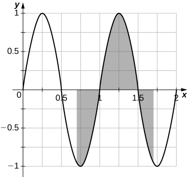
a. The graph is antisymmetric with respect to \(\displaystyle t=\frac{1}{2}\) over \(\displaystyle [0,1]\), so the average value is zero. b. For any value of a, the graph between \(\displaystyle [a,a+1]\) is a shift of the graph over \(\displaystyle [0,1]\), so the net areas above and below the axis do not change and the average remains zero.

83) If f is 1-periodic \(\displaystyle (f(t+1)=f(t))\), odd, and integrable over \(\displaystyle [0,1]\), is it always true that \(\displaystyle ∫^1_0f(t)dt=0?\)

84) If f is 1-periodic and \(\displaystyle ∫10f(t)dt=A,\) is it necessarily true that \(\displaystyle ∫^{1+a}_af(t)dt=A\) for all A?

Solution: Yes, the integral over any interval of length 1 is the same.

5.3: The Fundamental Theorem of Calculus

1) Consider two athletes running at variable speeds \(\displaystyle v_1(t)\) and \(\displaystyle v_2(t).\) The runners start and finish a race at exactly the same time. Explain why the two runners must be going the same speed at some point.

2) Two mountain climbers start their climb at base camp, taking two different routes, one steeper than the other, and arrive at the peak at exactly the same time. Is it necessarily true that, at some point, both climbers increased in altitude at the same rate?

Solution: Yes. It is implied by the Mean Value Theorem for Integrals.

3) To get on a certain toll road a driver has to take a card that lists the mile entrance point. The card also has a timestamp. When going to pay the toll at the exit, the driver is surprised to receive a speeding ticket along with the toll. Explain how this can happen.

4) Set \(\displaystyle F(x)=∫^x -1(1−t)dt.\) Find \(\displaystyle F′(2)\) and the average value of \(\displaystyle F'\) over \(\displaystyle [1,2].\)

Solution: \(\displaystyle F′(2)=−1;\) average value of \(\displaystyle F'\) over \(\displaystyle [1,2]\) is \(\displaystyle −1/2.\)

In the following exercises, use the Fundamental Theorem of Calculus, Part 1, to find each derivative.

5) \(\displaystyle \frac{d}{dx}∫^x_1e^{−t^2}dt\)

6) \(\displaystyle \frac{d}{dx}∫^x_1e^{cost}dt\)

Solution: \(\displaystyle e^{cost}\)

7) \(\displaystyle \frac{d}{dx}∫^x_3\sqrt{9−y^2}dy\)

8) \(\displaystyle \frac{d}{dx}∫^x_4\frac{ds}{\sqrt{16−s^2}}\)

Solution: \(\displaystyle \frac{1}{\sqrt{16−x^2}}\)

9) \(\displaystyle \frac{d}{dx}∫^{2x}x_tdt\)

10) \(\displaystyle \frac{d}{dx}∫^{\sqrt{x}}_0tdt\)

Solution: \(\displaystyle \sqrt{x}\frac{d}{dx}\sqrt{x}=\frac{1}{2}\)

11) \(\displaystyle \frac{d}{dx}∫^{sinx}_0\sqrt{1−t^2}dt\)

12) \(\displaystyle \frac{d}{dx}∫^1_{cosx}\sqrt{1−t^2}dt\)

Solution: \(\displaystyle −\sqrt{1−cos^2x}\frac{d}{dx}cosx=|sinx|sinx\)

13) \(\displaystyle \frac{d}{dx}∫^{\sqrt{x}}_1\frac{t^2}{1+t^4}dt\)

14) \(\displaystyle \frac{d}{dx}∫^{x^2}_1\frac{\sqrt{t}}{1+t}dt\)

Solution: \(\displaystyle 2x\frac{|x|}{1+x^2}\)

15) \(\displaystyle \frac{d}{dx}∫^{lnx}_0e^tdt\)

16) \(\displaystyle \frac{d}{dx}∫^{e^2}_1lnu^2du\)

Solution: \(\displaystyle ln(e^{2x})\frac{d}{dx}e^x=2xe^x\)

17) The graph of \(\displaystyle y=∫^x_0f(t)dt\), where f is a piecewise constant function, is shown here.

a. Over which intervals is f positive? Over which intervals is it negative? Over which intervals, if any, is it equal to zero?

b. What are the maximum and minimum values of f?

c. What is the average value of f?

18) The graph of \(\displaystyle y=∫^x_0f(t)dt\), where f is a piecewise constant function, is shown here.

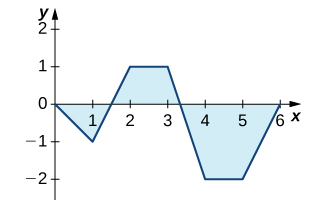
a. Over which intervals is f positive? Over which intervals is it negative? Over which intervals, if any, is it equal to zero?

b. What are the maximum and minimum values of f?

c. What is the average value of f?

Solution: a. f is positive over \(\displaystyle [1,2]\) and \(\displaystyle [5,6]\), negative over \(\displaystyle [0,1]\) and \(\displaystyle [3,4]\), and zero over \(\displaystyle [2,3]\) and \(\displaystyle [4,5]\). b. The maximum value is 2 and the minimum is −3. c. The average value is 0.

19) The graph of \(\displaystyle y=∫^x_0ℓ(t)dt\), where \(\displaystyle ℓ\) is a piecewise linear function, is shown here.

a. Over which intervals is ℓ positive? Over which intervals is it negative? Over which, if any, is it zero?

b. Over which intervals is ℓ increasing? Over which is it decreasing? Over which, if any, is it constant?

c. What is the average value of ℓ?

20) The graph of \(\displaystyle y=∫^x_0ℓ(t)dt\), where \(\displaystyle ℓ\) is a piecewise linear function, is shown here.

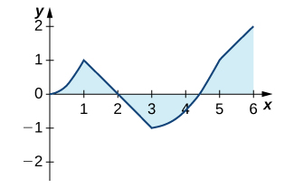
a. Over which intervals is ℓ positive? Over which intervals is it negative? Over which, if any, is it zero?

b. Over which intervals is ℓ increasing? Over which is it decreasing? Over which intervals, if any, is it constant?

c. What is the average value of ℓ?

Solution: a. ℓ is positive over \(\displaystyle [0,1]\) and \(\displaystyle [3,6]\), and negative over \(\displaystyle [1,3]\). b. It is increasing over \(\displaystyle [0,1]\) and \(\displaystyle [3,5]\), and it is constant over \(\displaystyle [1,3]\) and \(\displaystyle [5,6]\). c. Its average value is \(\displaystyle \frac{1}{3}\).

In the following exercises, use a calculator to estimate the area under the curve by computing \(\displaystyle T_{10}\), the average of the left- and right-endpoint Riemann sums using \(\displaystyle N=10\) rectangles. Then, using the Fundamental Theorem of Calculus, Part 2, determine the exact area.

21) [T] \(\displaystyle y=x^2\) over \(\displaystyle [0,4]\)

22) [T] \(\displaystyle y=x^3+6x^2+x−5\) over \(\displaystyle [−4,2]\)

Solution: \(\displaystyle T_{10}=49.08,∫^3_{−2}x^3+6x^2+x−5dx=48\)

23) [T] \(\displaystyle y=\sqrt{x^3}\) over \(\displaystyle [0,6]\)

24) [T] \(\displaystyle y=\sqrt{x}+x^2\) over \(\displaystyle [1,9]\)

Solution: \(\displaystyle T_{10}=260.836,∫^9_1(\sqrt{x}+x^2)dx=260\)

25) [T] \(\displaystyle ∫(cosx−sinx)dx\) over \(\displaystyle [0,π]\)

26) [T] \(\displaystyle ∫\frac{4}{x^2}dx\) over \(\displaystyle [1,4]\)

Solution: \(\displaystyle T_{10}=3.058,∫^4_1\frac{4}{x^2}dx=3\)

In the following exercises, evaluate each definite integral using the Fundamental Theorem of Calculus, Part 2.

27) \(\displaystyle ∫^2_{−1}(x^2−3x)dx\)

28) \(\displaystyle ∫^3_{−2}(x^2+3x−5)dx\)

Solution: \(\displaystyle F(x)=\frac{x^3}{3}+\frac{3x^2}{2}−5x,F(3)−F(−2)=−\frac{35}{6}\)

29) \(\displaystyle ∫^3_{−2}(t+2)(t−3)dt\)

30) \(\displaystyle ∫^3_2(t^2−9)(4−t^2)dt\)

Solution: \(\displaystyle F(x)=−\frac{t^5}{5}+\frac{13t^3}{3}−36t,F(3)−F(2)=\frac{62}{15}\)

31) \(\displaystyle ∫^2_1x^9dx\)

32) \(\displaystyle ∫^1_0x^{99}dx\)

Solution: \(\displaystyle F(x)=\frac{x^{100}}{100},F(1)−F(0)=\frac{1}{100}\)

33) \(\displaystyle ∫^8_4(4t^{5/2}−3t^{3/2})dt\)

34) \(\displaystyle ∫^4_{1/4}(x^2−\frac{1}{x^2})dx\)

Solution: \(\displaystyle F(x)=\frac{x^3}{3}+1\frac{x}{,}F(4)−F(\frac{1}{4})=\frac{1125}{64}\)

35) \(\displaystyle ∫^2_1\frac{2}{x^3}dx\)

36) \(\displaystyle ∫^4_1\frac{1}{2\sqrt{x}}dx\)

Solution: \(\displaystyle F(x)=\sqrt{x},F(4)−F(1)=1\)

37) \(\displaystyle ∫^4_1\frac{2−\sqrt{t}}{t^2}dt\)

38) \(\displaystyle ∫^{16}_1\frac{dt}{t^{1/4}}\)

Solution: \(\displaystyle F(x)=\frac{4}{3}t^{3/4},F(16)−F(1)=\frac{28}{3}\)

39) \(\displaystyle ∫^{2π}_0cosθdθ\)

40) \(\displaystyle ∫^{π/2}_0sinθdθ\)

Solution: \(\displaystyle F(x)=−cosx,F(\frac{π}{2})−F(0)=1\)

41) \(\displaystyle ∫^{π/4}_0sec^2θdθ\)

42) \(\displaystyle ∫^{π/4}_0secθtanθ\)

Solution: \(\displaystyle F(x)=secx,F(\frac{π}{4})−F(0)=\sqrt{2}−1\)

43) \(\displaystyle ∫^{π/4}_{π/3}cscθcotθdθ\)

44) \(\displaystyle (∫^{π/2}_{π/4}csc^2θdθ\)

Solution: \(\displaystyle F(x)=−cot(x),F(\frac{π}{2})−F(\frac{π}{4})=1\)

45) \(\displaystyle ∫^2_1(\frac{1}{t^2}−\frac{1}{t^3})dt\)

46) \(\displaystyle ∫^{−1}_{−2}(\frac{1}{t^2}−\frac{1}{t^3})dt\)

Solution: \(\displaystyle F(x)=−\frac{1}{x}+\frac{1}{2x^2},F(−1)−F(−2)=\frac{7}{8}\)

In the following exercises, use the evaluation theorem to express the integral as a function \(\displaystyle F(x).\)

47) \(\displaystyle ∫^x_at^2dt\)

48) \(\displaystyle ∫^x_1e^tdt\)

Solution: \(\displaystyle F(x)=e^x−e\)

49) \(\displaystyle ∫^x_0costdt\)

50) \(\displaystyle ∫^x_{−x}sintdt\)

Solution: \(\displaystyle F(x)=0\)

In the following exercises, identify the roots of the integrand to remove absolute values, then evaluate using the Fundamental Theorem of Calculus, Part 2.

51) \(\displaystyle ∫^3_{−2}|x|dx\)

52) \(\displaystyle ∫^4_{−2}∣t^2−2t−3∣dt\)

Solution: \(\displaystyle ∫^{−1}_{−2}(t^2−2t−3)dt−∫^3_{−1}(t^2−2t−3)dt+∫^4_3(t^2−2t−3)dt=\frac{46}{3}\)

53) \(\displaystyle ∫^π_0|cost|dt\)

54) \(\displaystyle ∫^{π/2}_{−π/2}|sint|dt\)

Solutionn: \(\displaystyle −∫^0_{−π/2}sintdt+∫^{π/2}_0sintdt=2\)

55) Suppose that the number of hours of daylight on a given day in Seattle is modeled by the function \(\displaystyle −3.75cos(\frac{πt}{6})+12.25\), with t given in months and \(\displaystyle t=0\) corresponding to the winter solstice.

a. What is the average number of daylight hours in a year?

b. At which times \(\displaystyle t_1\) and \(\displaystyle t_2\), where \(\displaystyle 0≤t_1<t_2<12,\) do the number of daylight hours equal the average number?

c. Write an integral that expresses the total number of daylight hours in Seattle between \(\displaystyle t_1\) and \(\displaystyle t_2\)

d. Compute the mean hours of daylight in Seattle between \(\displaystyle t_1\) and \(\displaystyle t_2\), where \(\displaystyle 0≤t_1<t_2<12\), and then between \(\displaystyle t_2\) and \(\displaystyle t_1\), and show that the average of the two is equal to the average day length.

56) Suppose the rate of gasoline consumption in the United States can be modeled by a sinusoidal function of the form \(\displaystyle (11.21−cos(\frac{πt}{6}))×10^9\) gal/mo.

a. What is the average monthly consumption, and for which values of t is the rate at time t equal to the average rate?

b. What is the number of gallons of gasoline consumed in the United States in a year?

c. Write an integral that expresses the average monthly U.S. gas consumption during the part of the year between the beginning of April \(\displaystyle (t=3)\) and the end of September \(\displaystyle (t=9).\)

Solution: a. The average is \(\displaystyle 11.21×10^9\) since \(\displaystyle cos(\frac{πt}{6})\) has period 12 and integral 0 over any period. Consumption is equal to the average when \(\displaystyle cos(\frac{πt}{6})=0\), when \(\displaystyle t=3\), and when \(\displaystyle t=9\). b. Total consumption is the average rate times duration: \(\displaystyle 11.21×12×10^9=1.35×10^{11}\) c. \(\displaystyle 10^9(11.21−\frac{1}{6}∫^9_3cos(\frac{πt}{6})dt)=10^9(11.21+2π)=11.84x10^9\)

57) Explain why, if f is continuous over \(\displaystyle [a,b],\) there is at least one point \(\displaystyle c∈[a,b]\) such that \(\displaystyle f(c)=\frac{1}{b−a}∫^b_af(t)dt.\)

58) Explain why, if f is continuous over \(\displaystyle [a,b]\) and is not equal to a constant, there is at least one point \(\displaystyle M∈[a,b]\) such that \(\displaystyle f(M)=\frac{1}{b−a}∫^b_af(t)dt\) and at least one point \(\displaystyle m∈[a,b]\) such that \(\displaystyle f(m)<\frac{1}{b−a}∫^b_af(t)dt\).

Solution: If f is not constant, then its average is strictly smaller than the maximum and larger than the minimum, which are attained over \(\displaystyle [a,b]\) by the extreme value theorem.

59) Kepler’s first law states that the planets move in elliptical orbits with the Sun at one focus. The closest point of a planetary orbit to the Sun is called the perihelion (for Earth, it currently occurs around January 3) and the farthest point is called the aphelion (for Earth, it currently occurs around July 4). Kepler’s second law states that planets sweep out equal areas of their elliptical orbits in equal times. Thus, the two arcs indicated in the following figure are swept out in equal times. At what time of year is Earth moving fastest in its orbit? When is it moving slowest?Kepler’s first law states that the planets move in elliptical orbits with the Sun at one focus. The closest point of a planetary orbit to the Sun is called the perihelion (for Earth, it currently occurs around January 3) and the farthest point is called the aphelion (for Earth, it currently occurs around July 4). Kepler’s second law states that planets sweep out equal areas of their elliptical orbits in equal times. Thus, the two arcs indicated in the following figure are swept out in equal times. At what time of year is Earth moving fastest in its orbit? When is it moving slowest?

60) A point on an ellipse with major axis length 2a and minor axis length 2b has the coordinates \(\displaystyle (acosθ,bsinθ),0≤θ≤2π.\)

a. Show that the distance from this point to the focus at \(\displaystyle (−c,0)\) is \(\displaystyle d(θ)=a+ccosθ\), where \(\displaystyle c=\sqrt{a^2−b^2}\).

Use these coordinates to show that the average distance \(\displaystyle \bar{d}\) from a point on the ellipse to the focus at \(\displaystyle (−c,0),\) with respect to angle θ, is a.

Solution: \(\displaystyle a. d^2θ=(acosθ+c)^2+b^2sin^2θ=a^2+c^2cos^2θ+2accosθ=(a+ccosθ)^2;\)

\(\displaystyle b. \bar{d}=\frac{1}{2π}∫^{2π}_0(a+2ccosθ)dθ=a\)

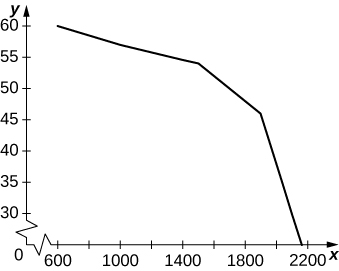
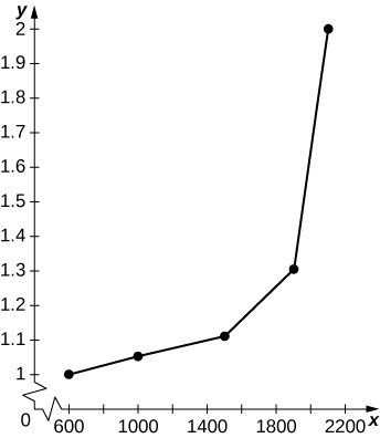
61) As implied earlier, according to Kepler’s laws, Earth’s orbit is an ellipse with the Sun at one focus. The perihelion for Earth’s orbit around the Sun is 147,098,290 km and the aphelion is 152,098,232 km.

a. By placing the major axis along the x-axis, find the average distance from Earth to the Sun.

b. The classic definition of an astronomical unit (AU) is the distance from Earth to the Sun, and its value was computed as the average of the perihelion and aphelion distances. Is this definition justified?

62) The force of gravitational attraction between the Sun and a planet is \(\displaystyle F(θ)=\frac{GmM}{r^2(θ)}\), where m is the mass of the planet, M is the mass of the Sun, G is a universal constant, and \(\displaystyle r(θ)\) is the distance between the Sun and the planet when the planet is at an angle θ with the major axis of its orbit. Assuming that M, m, and the ellipse parameters a and b (half-lengths of the major and minor axes) are given, set up—but do not evaluate—an integral that expresses in terms of \(\displaystyle G,m,M,a,b\) the average gravitational force between the Sun and the planet.

Solution: Mean gravitational force \(\displaystyle = \frac{GmM}{2}∫^{2π}_0\frac{1}{(a+2\sqrt{a^2−b^2}cosθ)^2}dθ\).

The displacement from rest of a mass attached to a spring satisfies the simple harmonic motion equation \(\displaystyle x(t)=Acos(ωt−ϕ),\) where \(\displaystyle ϕ\) is a phase constant, ω is the angular frequency, and A is the amplitude. Find the average velocity, the average speed (magnitude of velocity), the average displacement, and the average distance from rest (magnitude of displacement) of the mass.

5.4: Integration Formulas and the Net Change Theorem

Use basic integration formulas to compute the following antiderivatives.

1) \(\displaystyle ∫(\sqrt{x}−\frac{1}{\sqrt{x}})dx\)

Solution: \(\displaystyle ∫(\sqrt{x}−\frac{1}{\sqrt{x}})dx=∫x^{1/2}dx−∫x^{−1/2}dx=\frac{2}{3}x^{3/2}+C_1−2x^{1/2+}C_2=\frac{2}{3}x^{3/2}−2x^{1/2}+C\)

2) \(\displaystyle ∫(e^{2x}−\frac{1}{2}e^{x/2})dx\)

3) \(\displaystyle ∫\frac{dx}{2x}\)

Solution: \(\displaystyle ∫\frac{dx}{2x}=\frac{1}{2}ln|x|+C\)

4) \(\displaystyle ∫\frac{x−1}{x^2}dx\)

5) \(\displaystyle ∫^π_0(sinx−cosx)dx\)

Solution: \(\displaystyle ∫^π_0sinxdx−∫^π_0cosxdx=−cosx|^π_0−(sinx)|^π_0=(−(−1)+1)−(0−0)=2\)

6) \(\displaystyle ∫^{π/2}_0(x−sinx)dx\)

7) Write an integral that expresses the increase in the perimeter \(\displaystyle P(s)\) of a square when its side length s increases from 2 units to 4 units and evaluate the integral.

Solution: \(\displaystyle P(s)=4s,\) so \(\displaystyle \frac{dP}{ds}=4\) and \(\displaystyle ∫^4_24ds=8.\)

8) Write an integral that quantifies the change in the area \(\displaystyle A(s)=s^2\)of a square when the side length doubles from S units to 2S units and evaluate the integral.

9) A regular N-gon (an N-sided polygon with sides that have equal length s, such as a pentagon or hexagon) has perimeter Ns. Write an integral that expresses the increase in perimeter of a regular N-gon when the length of each side increases from 1 unit to 2 units and evaluate the integral.

Solution: \(\displaystyle ∫^2_1Nds=N\)

10) The area of a regular pentagon with side length \(\displaystyle a>0\) is \(\displaystyle pa^2\) with \(\displaystyle p=\frac{1}{4}\sqrt{5+\sqrt{5+2\sqrt{5}}}\). The Pentagon in Washington, DC, has inner sides of length 360 ft and outer sides of length 920 ft. Write an integral to express the area of the roof of the Pentagon according to these dimensions and evaluate this area.

11) A dodecahedron is a Platonic solid with a surface that consists of 12 pentagons, each of equal area. By how much does the surface area of a dodecahedron increase as the side length of each pentagon doubles from 1 unit to 2 units?

Solution: With p as in the previous exercise, each of the 12 pentagons increases in area from 2p to 4p units so the net increase in the area of the dodecahedron is 36punits.

12) An icosahedron is a Platonic solid with a surface that consists of 20 equilateral triangles. By how much does the surface area of an icosahedron increase as the side length of each triangle doubles from a unit to 2a units?

13) Write an integral that quantifies the change in the area of the surface of a cube when its side length doubles from s unit to 2s units and evaluate the integral.

Solution: \(\displaystyle 18s^2=6∫^{2s}_s2xdx\)

14) Write an integral that quantifies the increase in the volume of a cube when the side length doubles from s unit to 2s units and evaluate the integral.

15) Write an integral that quantifies the increase in the surface area of a sphere as its radius doubles from R unit to 2R units and evaluate the integral.

Solution: \(\displaystyle 12πR^2=8π∫^{2R}_Rrdr\)

16) Write an integral that quantifies the increase in the volume of a sphere as its radius doubles from R unit to 2R units and evaluate the integral.

17) Suppose that a particle moves along a straight line with velocity \(\displaystyle v(t)=4−2t,\) where \(\displaystyle 0≤t≤2\) (in meters per second). Find the displacement at time t and the total distance traveled up to \(\displaystyle t=2.\)

Solution: \(\displaystyle d(t)=∫^t_0v(s)ds=4t−t^2\). The total distance is \(\displaystyle d(2)=4m.\)

18) Suppose that a particle moves along a straight line with velocity defined by \(\displaystyle v(t)=t^2−3t−18,\) where \(\displaystyle 0≤t≤6\) (in meters per second). Find the displacement at time t and the total distance traveled up to \(\displaystyle t=6.\)

19) Suppose that a particle moves along a straight line with velocity defined by \(\displaystyle v(t)=|2t−6|,\) where \(\displaystyle 0≤t≤6\) (in meters per second). Find the displacement at time t and the total distance traveled up to \(\displaystyle t=6.\)

Solution: \(\displaystyle d(t)=∫^t_0v(s)ds.\) For \(\displaystyle t<3,d(t)=∫^t_0(6−2t)dt=6t−t^2\). For \(\displaystyle t>3,d(t)=d(3)+∫^t_3(2t−6)dt=9+(t^2−6t)\). The total distance is \(\displaystyle d(6)=9m.\)

20) Suppose that a particle moves along a straight line with acceleration defined by \(\displaystyle a(t)=t−3,\) where \(\displaystyle 0≤t≤6\) (in meters per second). Find the velocity and displacement at time t and the total distance traveled up to \(\displaystyle t=6\) if \(\displaystyle v(0)=3\) and \(\displaystyle d(0)=0.\)

21) A ball is thrown upward from a height of 1.5 m at an initial speed of 40 m/sec. Acceleration resulting from gravity is −9.8 m/sec2. Neglecting air resistance, solve for the velocity \(\displaystyle v(t)\) and the height \(\displaystyle h(t)\) of the ball t seconds after it is thrown and before it returns to the ground.

Solution: \(\displaystyle v(t)=40−9.8t;h(t)=1.5+40t−4.9t^2\)m/s

22) A ball is thrown upward from a height of 3 m at an initial speed of 60 m/sec. Acceleration resulting from gravity is \(\displaystyle −9.8 m/sec^2\). Neglecting air resistance, solve for the velocity \(\displaystyle v(t)\) and the height \(\displaystyle h(t)\) of the ball t seconds after it is thrown and before it returns to the ground.

23) The area \(\displaystyle A(t)\) of a circular shape is growing at a constant rate. If the area increases from 4π units to 9π units between times \(\displaystyle t=2\) and \(\displaystyle t=3,\) find the net change in the radius during that time.

Solution: The net increase is 1 unit.

24) A spherical balloon is being inflated at a constant rate. If the volume of the balloon changes from \(\displaystyle 36π in.^3\) to \(\displaystyle 288π in.^3\) between time \(\displaystyle t=30\) and \(\displaystyle t=60\) seconds, find the net change in the radius of the balloon during that time.

25) Water flows into a conical tank with cross-sectional area \(\displaystyle πx^2\) at height x and volume \(\displaystyle \frac{πx^3}{3}\) up to height x. If water flows into the tank at a rate of 1 \(\displaystyle m^3/min\), find the height of water in the tank after 5 min. Find the change in height between 5 min and 10 min.

Solution: At \(\displaystyle t=5\), the height of water is \(\displaystyle x=(\frac{15}{π})^{1/3}m..\) The net change in height from \(\displaystyle t=5\) to \(\displaystyle t=10\) is \(\displaystyle (\frac{(30}{π})^{1/3}−(\frac{15}{π})^{1/3}m.\)

26) A horizontal cylindrical tank has cross-sectional area \(\displaystyle A(x)=4(6x−x^2)m^2\) at height x meters above the bottom when \(\displaystyle x≤3.\)

a. The volume V between heights a and b is \(\displaystyle ∫^b_aA(x)dx.\) Find the volume at heights between 2 m and 3 m.

b. Suppose that oil is being pumped into the tank at a rate of 50 L/min. Using the chain rule, \(\displaystyle \frac{dx}{dt}=\frac{dx}{dV}\frac{dV}{dt}\), at how many meters per minute is the height of oil in the tank changing, expressed in terms of x, when the height is at x meters?

c. How long does it take to fill the tank to 3 m starting from a fill level of 2 m?

27) The following table lists the electrical power in gigawatts—the rate at which energy is consumed—used in a certain city for different hours of the day, in a typical 24-hour period, with hour 1 corresponding to midnight to 1 a.m.

Hour	Power	Hour	Power
1	28	13	48
2	25	14	49
3	24	15	49
4	23	16	50
5	24	17	50
6	27	18	50
7	29	19	46
8	32	20	43
9	34	21	42
10	39	22	40
11	42	23	37
12	46	24	34

Find the total amount of power in gigawatt-hours (gW-h) consumed by the city in a typical 24-hour period.

Solution: The total daily power consumption is estimated as the sum of the hourly power rates, or 911 gW-h.

28) The average residential electrical power use (in hundreds of watts) per hour is given in the following table.

Hour	Power	Hour	Power
1	8	13	12
2	6	14	13
3	5	15	14
4	4	16	15
5	5	17	17
6	6	18	19
7	7	19	18
8	8	20	17
9	9	21	16
10	10	22	16
11	10	23	13
12	11	24	11

a. Compute the average total energy used in a day in kilowatt-hours (kWh).

b. If a ton of coal generates 1842 kWh, how long does it take for an average residence to burn a ton of coal?

c. Explain why the data might fit a plot of the form \(\displaystyle p(t)=11.5−7.5sin(\frac{πt}{12}).\)

29) The data in the following table are used to estimate the average power output produced by Peter Sagan for each of the last 18 sec of Stage 1 of the 2012 Tour de France.

Second	Watts	Second	Watts
1	600	10	1200
2	500	11	1170
3	575	12	1125
4	1050	13	1100
5	925	14	1075
6	950	15	1000
7	1050	16	950
8	950	17	900
9	1100	18	780

Average Power OutputSource: sportsexercisengineering.com

Estimate the net energy used in kilojoules (kJ), noting that 1W = 1 J/s, and the average power output by Sagan during this time interval.

Solution: 17 kJ

30) The data in the following table are used to estimate the average power output produced by Peter Sagan for each 15-min interval of Stage 1 of the 2012 Tour de France.

Minutes	Watts	Minutes	Watts
15	200	165	170
30	180	180	220
45	190	195	140
60	230	210	225
75	240	225	170
90	210	240	10
105	210	255	200
1120	220	270	220
135	210	285	250
150	150	300	400

Average Power OutputSource: sportsexercisengineering.com

Estimate the net energy used in kilojoules, noting that 1W = 1 J/s.

31) The distribution of incomes as of 2012 in the United States in $5000 increments is given in the following table. The kth row denotes the percentage of households with incomes between \(\displaystyle $5000xk\) and \(\displaystyle 5000xk+4999\). The row \(\displaystyle k=40\) contains all households with income between $200,000 and $250,000 and \(\displaystyle k=41\) accounts for all households with income exceeding $250,000.

0	3.5	21	1.5
1	4.1	22	1.4
2	5.9	23	1.3
3	5.7	24	1.3
4	5.9	25	1.1
5	5.4	26	1.0
6	5.5	27	0.75
7	5.1	28	0.8
8	4.8	29	1.0
9	4.1	30	0.6
10	4.3	31	0.6
11	3.5	32	.5
12	3.7	33	0.5
13	3.2	34	0.4
14	3.0	35	0.3
15	2.8	36	0.3
16	2.5	37	0.3
17	2.2	38	0.2
18	2.2	39	1.8
19	1.8	40	2.3
20	2.1	41

Income DistributionsSource: http://www.census.gov/prod/2013pubs/p60-245.pdf

a. Estimate the percentage of U.S. households in 2012 with incomes less than $55,000.

b. What percentage of households had incomes exceeding $85,000?

c. Plot the data and try to fit its shape to that of a graph of the form \(\displaystyle a(x+c)e^{−b(x+e)}\) for suitable \(\displaystyle a,b,c.\)

Solution: \(\displaystyle a. 54.3%; b. 27.00%; c. \)The curve in the following plot is \(\displaystyle 2.35(t+3)e^{−0.15(t+3)}.\)

32) Newton’s law of gravity states that the gravitational force exerted by an object of mass M and one of mass m with centers that are separated by a distance r is \(\displaystyle F=G\frac{mM}{r^2}\), with G an empirical constant \(\displaystyle G=6.67x10^{−11}m^3/(kg⋅s^2)\). The work done by a variable force over an interval \(\displaystyle [a,b]\) is defined as \(\displaystyle W=∫^b_aF(x)dx\). If Earth has mass \(\displaystyle 5.97219×10^{24}\) and radius 6371 km, compute the amount of work to elevate a polar weather satellite of mass 1400 kg to its orbiting altitude of 850 km above Earth.

33) For a given motor vehicle, the maximum achievable deceleration from braking is approximately 7 m/sec2 on dry concrete. On wet asphalt, it is approximately 2.5 m/sec2. Given that 1 mph corresponds to 0.447 m/sec, find the total distance that a car travels in meters on dry concrete after the brakes are applied until it comes to a complete stop if the initial velocity is 67 mph (30 m/sec) or if the initial braking velocity is 56 mph (25 m/sec). Find the corresponding distances if the surface is slippery wet asphalt.

Solution: In dry conditions, with initial velocity \(\displaystyle v_0=30\) m/s, \(\displaystyle D=64.3\) and, if \(\displaystyle v_0=25,D=44.64\). In wet conditions, if \(\displaystyle v_0=30\), and \(\displaystyle D=180\) and if \(\displaystyle v_0=25,D=125.\)

34) John is a 25-year old man who weighs 160 lb. He burns \(\displaystyle 500−50t\) calories/hr while riding his bike for t hours. If an oatmeal cookie has 55 cal and John eats 4t cookies during the tth hour, how many net calories has he lost after 3 hours riding his bike?

35) Sandra is a 25-year old woman who weighs 120 lb. She burns \(\displaystyle 300−50t\) cal/hr while walking on her treadmill. Her caloric intake from drinking Gatorade is 100t calories during the tth hour. What is her net decrease in calories after walking for 3 hours?

Solution: 225 cal

36) A motor vehicle has a maximum efficiency of 33 mpg at a cruising speed of 40 mph. The efficiency drops at a rate of 0.1 mpg/mph between 40 mph and 50 mph, and at a rate of 0.4 mpg/mph between 50 mph and 80 mph. What is the efficiency in miles per gallon if the car is cruising at 50 mph? What is the efficiency in miles per gallon if the car is cruising at 80 mph? If gasoline costs $3.50/gal, what is the cost of fuel to drive 50 mi at 40 mph, at 50 mph, and at 80 mph?

37) Although some engines are more efficient at given a horsepower than others, on average, fuel efficiency decreases with horsepower at a rate of \(\displaystyle 1/25\) mpg/horsepower. If a typical 50-horsepower engine has an average fuel efficiency of 32 mpg, what is the average fuel efficiency of an engine with the following horsepower: 150, 300, 450?

Solution: \(\displaystyle E(150)=28,E(300)=22,E(450)=16\)

38) [T] The following table lists the 2013 schedule of federal income tax versus taxable income.

Taxable Income Range	The Tax Is ...	... Of the Amount Over
$0–$8925	10%	$0
$8925–$36,250	$892.50 + 15%	$8925
$36,250–$87,850	$4,991.25 + 25%	$36,250
$87,850–$183,250	$17,891.25 + 28%	$87,850
$183,250–$398,350	$44,603.25 + 33%	$183,250
$398,350–$400,000	$115,586.25 + 35%	$398,350
> $400,000	$116,163.75 + 39.6%	$400,000

Federal Income Tax Versus Taxable IncomeSource: http://www.irs.gov/pub/irs-prior/i1040tt--2013.pdf.

Suppose that Steve just received a $10,000 raise. How much of this raise is left after federal taxes if Steve’s salary before receiving the raise was $40,000? If it was $90,000? If it was $385,000?

39) [T] The following table provides hypothetical data regarding the level of service for a certain highway.

Highway Speed Range (mph)	Vehicles per Hour per Lane	Density Range (vehicles/mi)
>60	<600	<10
60-57	300-1000	10-20
57-54	1000-1500	20-30
57-54	1500-1900	30-45
46-30	1900-2100	48-70
<30	Unstable	70-200

a. Plot vehicles per hour per lane on the x-axis and highway speed on the y-axis.

b. Compute the average decrease in speed (in miles per hour) per unit increase in congestion (vehicles per hour per lane) as the latter increases from 600 to 1000, from 1000 to 1500, and from 1500 to 2100. Does the decrease in miles per hour depend linearly on the increase in vehicles per hour per lane?

c. Plot minutes per mile (60 times the reciprocal of miles per hour) as a function of vehicles per hour per lane. Is this function linear?

Solution:

a.

b. Between 600 and 1000 the average decrease in vehicles per hour per lane is −0.0075. Between 1000 and 1500 it is −0.006 per vehicles per hour per lane, and between 1500 and 2100 it is −0.04 vehicles per hour per lane. c.

The graph is nonlinear, with minutes per mile increasing dramatically as vehicles per hour per lane reach 2000.

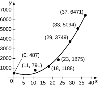
40) For the next two exercises use the data in the following table, which displays bald eagle populations from 1963 to 2000 in the continental United States.

Year	Population of Breeding Pairs of Bald Eagles
1963	487
1974	791
1981	1188
1986	1875
1992	3749
1996	5094
2000	6471

Population of Breeding Bald Eagle PairsSource: http://www.fws.gov/Midwest/eagle/pop.../chtofprs.html.

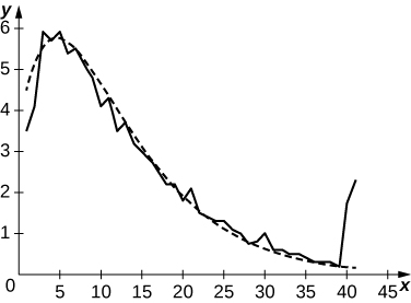
41) [T] The graph below plots the quadratic \(\displaystyle p(t)=6.48t^2−80.31t+585.69\) against the data in preceding table, normalized so that \(\displaystyle t=0\) corresponds to 1963. Estimate the average number of bald eagles per year present for the 37 years by computing the average value of p over \(\displaystyle [0,37].\)

42) [T] The graph below plots the cubic \(\displaystyle p(t)=0.07t^3+2.42t^2−25.63t+521.23\) against the data in the preceding table, normalized so that \(\displaystyle t=0\) corresponds to 1963. Estimate the average number of bald eagles per year present for the 37 years by computing the average value of p over \(\displaystyle [0,37].\)

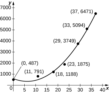
Solution: \(\displaystyle \frac{1}{37}∫^{37}_0p(t)dt=\frac{0.07(37)^3}{4}+\frac{2.42(37)^2}{3}−\frac{25.63(37)}{2}+521.23≈2037\)

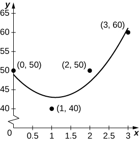
43) [T] Suppose you go on a road trip and record your speed at every half hour, as compiled in the following table. The best quadratic fit to the data is \(\displaystyle q(t)=5x^2−11x+49\), shown in the accompanying graph. Integrate q to estimate the total distance driven over the 3 hours.

Time (hr)	Speed (m[h)
0 (start)	50
1	40
2	50
3	60

As a car accelerates, it does not accelerate at a constant rate; rather, the acceleration is variable. For the following exercises, use the following table, which contains the acceleration measured at every second as a driver merges onto a freeway.

Time (sec)	Acceleration (mph/sex)
1	11.2
2	10.6
3	8.1
4	5.4
5	0

45) [T] The accompanying graph plots the best quadratic fit, \(\displaystyle a(t)=−0.70t^2+1.44t+10.44\), to the data from the preceding table. Compute the average value of a(t) to estimate the average acceleration between \(\displaystyle t=0\) and \(\displaystyle t=5.\)

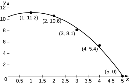
Solution: Average acceleration is \(\displaystyle A=\frac{1}{5}∫^5_0a(t)dt=−\frac{0.7(5^2)}{3}+\frac{1.44(5)}{2}+10.44≈8.2\) mph/s

46) [T] Using your acceleration equation from the previous exercise, find the corresponding velocity equation. Assuming the final velocity is 0 mph, find the velocity at time \(\displaystyle t=0.\)

47) [T] Using your velocity equation from the previous exercise, find the corresponding distance equation, assuming your initial distance is 0 mi. How far did you travel while you accelerated your car? (Hint: You will need to convert time units.)

Solution: \(\displaystyle d(t)=∫^1_0|v(t)|dt=∫^t_0(\frac{7}{30}t^3−0.72t^2−10.44t+41.033)dt=\frac{7}{120}t^4−0.24t^3−5.22t^3+41.033t.\) Then, \(\displaystyle d(5)≈81.12 mph ×sec≈119\) feet.

48) [T] The number of hamburgers sold at a restaurant throughout the day is given in the following table, with the accompanying graph plotting the best cubic fit to the data, \(\displaystyle b(t)=0.12t^3−2.13t^3+12.13t+3.91,\) with \(\displaystyle t=0\) corresponding to 9 a.m. and \(\displaystyle t=12\) corresponding to 9 p.m. Compute the average value of \(\displaystyle b(t)\) to estimate the average number of hamburgers sold per hour.

Hours Past Midnight	No. of Burgers Sold
9	3
12	28
15	20
18	30
21	45

49) [T] An athlete runs by a motion detector, which records her speed, as displayed in the following table. The best linear fit to this data, \(\displaystyle ℓ(t)=−0.068t+5.14\), is shown in the accompanying graph. Use the average value of \(\displaystyle ℓ(t)\) between \(\displaystyle t=\)0 and \(\displaystyle t=40\) to estimate the runner’s average speed.

Minutes	Speed (m/sec)
0	5
10	4.8
20	3.6
30	3.0
40	2.5

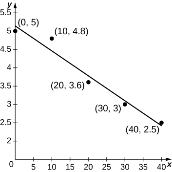
Solution: \(\displaystyle \frac{1}{40} ∫^{40}_0(−0.068t+5.14)dt=−\frac{0.068(40)}{2}+5.14=3.78\)

5.5: Substitution

1) Why is u-substitution referred to as change of variable?

2) 2. If \(\displaystylef=g∘h\), when reversing the chain rule, \(\displaystyle\frac{d}{d}x(g∘h)(x)=g′(h(x))h′(x)\), should you take \(\displaystyleu=g(x)\) or u= \(\displaystyleh(x)?\)

Solution: \(\displaystyleu=h(x)\)

In the following exercises, verify each identity using differentiation. Then, using the indicated u-substitution, identify f such that the integral takes the form \(\displaystyle∫f(u)du.\)

3) \(\displaystyle∫x\sqrt{x+1}x=\frac{2}{15}(x+1)^{3/2}(3x−2)+C;u=x+1\)

4) \(\displaystyle∫\frac{x^2}{\sqrt{x−1}}dx(x>1)=\frac{2}{15}\sqrt{x−1}(3x^2+4x+8)+C;u=x−1\)

Solution: \(\displaystylef(u)=\frac{(u+1)^2}{\sqrt{u}}\)

5) \(\displaystyle∫x\sqrt{4x^2+9}dx=\frac{1}{12}(4x^2+9)^{3/2}+C;u=4x^2+9\)

6) \(\displaystyle∫\frac{x}{\sqrt{4x^2+9}}dx=\frac{1}{4}\sqrt{4x^2+9}+C;u=4x^2+9\)

Solution: \(\displaystyledu=8xdx;f(u)=\frac{1}{8\sqrt{u}}\)

7) \(\displaystyle∫\frac{x}{(4x^2+9)^2}dx=−\frac{1}{8(4x^2+9)};u=4x^2+9\)

In the following exercises, find the antiderivative using the indicated substitution.

8) \(\displaystyle∫(x+1)^4dx;u=x+1\)

Solutio: \(\displaystyle\frac{1}{5}(x+1)^5+C\)

9) \(\displaystyle∫(x−1)^5dx;u=x−1\)

10) \(\displaystyle∫(2x−3)^{−7}dx;u=2x−3\)

Solution: \(\displaystyle−\frac{1}{12(3−2x)^6}+C\)

11) \(\displaystyle∫(3x−2)^{−11}dx;u=3x−2\)

12) \(\displaystyle∫\frac{x}{\sqrt{x^2+1}}dx;u=x^2+1\)

Solution: \(\displaystyle\sqrt{x^2+1}+C\)

13) \(\displaystyle∫\frac{x}{\sqrt{1−x^2}}dx;u=1−x^2\)

14) \(\displaystyle∫(x−1)(x^2−2x)^3dx;u=x^2−2x\)

Solution: \(\displaystyle\frac{1}{8}(x^2−2x)^4+C\)

15) \(\displaystyle∫(x^2−2x)(x^3−3x^2)^2dx;u=x^3=3x^2\)

16) \(\displaystyle∫cos^3θdθ;u=sinθ (Hint:cos^2θ=1−sin^2θ)\)

Solution: \( \sin θ−\frac{sin^3θ}{3}+C\)

17) \(\displaystyle∫sin^3θdθ;u=cosθ (Hint:sin^2θ=1−cos^2θ)\)

In the following exercises, use a suitable change of variables to determine the indefinite integral.

18) \(\displaystyle∫x(1−x)^{99}dx\)

Solution: \(\displaystyle\frac{(1−x)^{101}}{101}−\frac{(1−x)^{100}}{100}+C\)

19) \(\displaystyle∫t(1−t^2)^{10}dt\)

20) \(\displaystyle∫(11x−7)^{−3}dx\)

Solution: \(\displaystyle−\frac{1}{22(7−11x^2)}+C\)

21) \(\displaystyle∫(7x−11)^4dx\)

22) \(\displaystyle∫cos^3θsinθdθ\)

Solution: \(\displaystyle−\frac{cos^4θ}{4}+C\)

23) \(\displaystyle∫sin^7θcosθdθ\)

24) \(\displaystyle∫cos^2(πt)sin(πt)dt\)

Solution: \(\displaystyle−\frac{cos^3(πt)}{3π}+C\)

25) \(\displaystyle∫sin^2xcos^3xdx (Hint:sin^2x+cos^2x=1)\)

26) \(\displaystyle∫tsin(t^2)cos(t^2)dt\)

Solution: \(\displaystyle−\frac{1}{4}cos^2(t^2)+C\)

27) \(\displaystyle∫t^2cos^2(t^3)sin(t^3)dt\)

28) \(\displaystyle∫\frac{x^2}{(x^3−3)^2}dx\)

Solution: \(\displaystyle−\frac{1}{3(x^3−3)}+C\)

29) \(\displaystyle∫\frac{x^3}{\sqrt{1−x^2}}dx\)

30) \(\displaystyle∫\frac{y^5}{(1−y^3)^{3/2}}dy\)

Solution: \(\displaystyle−\frac{2(y^3−2)}{3\sqrt{1−y^3}}\)

31) \(\displaystyle∫cosθ(1−cosθ)^{99}sinθdθ\)

32) \(\displaystyle∫(1−cos^3θ)^{10}cos^2θsinθdθ\)

Solution: \(\displaystyle\frac{1}{33}(1−cos^3θ)^{11}+C\)

33) \(\displaystyle∫(cosθ−1)(cos^2θ−2cosθ)^3sinθdθ\)

34) \(\displaystyle∫(sin^2θ−2sinθ)(sin^3θ−3sin^2θ^)3cosθdθ\)

Solution: \(\displaystyle\frac{1}{12}(sin^3θ−3sin^2θ)^4+C\)

In the following exercises, use a calculator to estimate the area under the curve using left Riemann sums with 50 terms, then use substitution to solve for the exact answer.

35) [T] \(\displaystyley=3(1−x)^2\) over \(\displaystyle[0,2]\)

36) [T] \(\displaystyley=x(1−x^2)^3\) over \(\displaystyle[−1,2]\)

Solution: \(\displaystyleL_{50}=−8.5779.\) The exact area is \(\displaystyle\frac{−81}{8}\)

37) [T] \(\displaystyley=sinx(1−cosx)^2\) over \(\displaystyle[0,π]\)

38) [T] \(\displaystyley=\frac{x}{(x2^+1)^2}\) over \(\displaystyle[−1,1]\)

Solution: \(\displaystyleL_{50}=−0.006399\) … The exact area is 0.

In the following exercises, use a change of variables to evaluate the definite integral.

39) \(\displaystyle∫^1_0x\sqrt{1−x^2}dx\)

40) \(\displaystyle∫^1_0\frac{x}{\sqrt{1+x^2}}dx\)

Solution: \(\displaystyleu=1+x^2,du=2xdx,\frac{1}{2}∫^2_1u^{−1/2}du=\sqrt{2}−1\)

41) \(\displaystyle∫^2_0\frac{t}{\sqrt{5+t^2}}dt\)

42) \(\displaystyle∫^1_0\frac{t}{\sqrt{1+t^3}}dt\)

Solution: \(\displaystyleu=1+t^3,du=3t^2,\frac{1}{3}∫^2_1u^{−1/2}du=\frac{2}{3}(\sqrt{2}−1)\)

43) \(\displaystyle∫^{π/4}_0sec^2θtanθdθ\)

44) \(\displaystyle∫^{π/4}_0\frac{sinθ}{cos^4θ}dθ\)

Solution: \(\displaystyleu=cosθ,du=−sinθdθ,∫^1_{1/\sqrt{2}}u^{−4}du=\frac{1}{3}(2\sqrt{2}−1)\)

In the following exercises, evaluate the indefinite integral \(\displaystyle∫f(x)dx\) with constant \(\displaystyleC=0\) using u-substitution. Then, graph the function and the antiderivative over the indicated interval. If possible, estimate a value of C that would need to be added to the antiderivative to make it equal to the definite integral \(\displaystyleF(x)=∫^x_af(t)dt\), with a the left endpoint of the given interval.

45) [T] \(\displaystyle∫(2x+1)e^{x^2+x−6}dx\) over \(\displaystyle[−3,2]\)

46) [T] \(\displaystyle∫\frac{cos(ln(2x))}{x}dx\) on \(\displaystyle[0,2]\)

Solution:

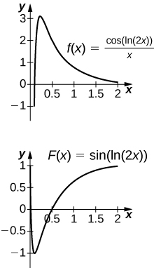
The antiderivative is \(\displaystyley=sin(ln(2x))\). Since the antiderivative is not continuous at \(\displaystylex=0\), one cannot find a value of C that would make \(\displaystyley=sin(ln(2x))−C\) work as a definite integral.

47) [T] \(\displaystyle∫\frac{3x^2+2x+1}{\sqrt{x^3+x^2+x+4}}dx\) over \(\displaystyle[−1,2]\)

48) [T] \(\displaystyle∫\frac{sinx}{cos^3x}dx\) over \(\displaystyle[−\frac{π}{3},\frac{π}{3}]\)

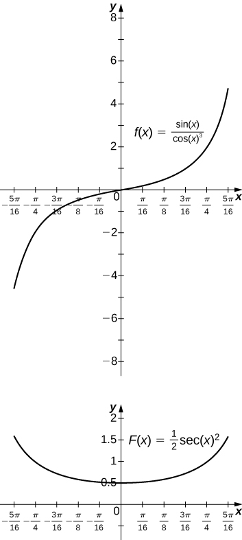
The antiderivative is \(\displaystyley=\frac{1}{2}sec^2x\). You should take \(\displaystyleC=−2\) so that \(\displaystyleF(−\frac{π}{3})=0.\)

49) [T] \(\displaystyle∫(x+2)e^{−x^2−4x+3}dx\) over \(\displaystyle[−5,1]\)

50) [T] \(\displaystyle∫3x^2\sqrt{2x^3+1}dx\) over \(\displaystyle[0,1]\)

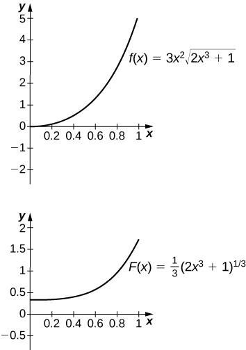
The antiderivative is \(\displaystyley=\frac{1}{3}(2x^3+1)^{3/2}\). One should take \(\displaystyleC=−\frac{1}{3}\).

51) If \(\displaystyleh(a)=h(b)\) in \(\displaystyle∫^b_ag'(h(x))h(x)dx,\) what can you say about the value of the integral?

52) Is the substitution \(\displaystyleu=1−x^2\) in the definite integral \(\displaystyle∫^2_0\frac{x}{1−x^2}dx\) okay? If not, why not?

Solution: No, because the integrand is discontinuous at \(\displaystylex=1\).

In the following exercises, use a change of variables to show that each definite integral is equal to zero.

53) \(\displaystyle∫^π_0cos^2(2θ)sin(2θ)dθ\)

54) \(\displaystyle∫^\sqrt{π}_0tcos(t^2)sin(t^2)dt\)

Solution: \(\displaystyleu=sin(t^2);\) the integral becomes \(\displaystyle\frac{1}{2}∫^0_0udu.\)

55) \(\displaystyle∫^1_0(1−2t)dt\)

56) \(\displaystyle∫^1_0\frac{1−2t}{(1+(t−\frac{1}{2})^2)}dt\)

Solution: \(\displaystyleu=(1+(t−\frac{1}{2})^2);\) the integral becomes \(\displaystyle−∫^{5/4}_{5/4}\frac{1}{u}du\).

57) \(\displaystyle∫^π_0sin((t−\frac{π}{2})^3)cos(t−\frac{π}{2})dt\)

58) \(\displaystyle∫^2_0(1−t)cos(πt)dt\)

Solution: \(\displaystyleu=1−t;\) the integral becomes

\(\displaystyle∫^{−1}_1ucos(π(1−u))du=∫^{−1}_1u[cosπcosu−sinπsinu]du=−∫^{−1}_1ucosudu=∫^{1−}_1ucosudu=0\)

since the integrand is odd.

59) \(\displaystyle∫^{3π/4}_{π/4}sin^2tcostdt\)

60) Show that the average value of \(\displaystylef(x)\) over an interval \(\displaystyle[a,b]\) is the same as the average value of \(\displaystylef(cx)\) over the interval \(\displaystyle[\frac{a}{c},\frac{b}{c}]\) for \(\displaystylec>0.\)

Solution: Setting \(\displaystyleu=cx\) and \(\displaystyledu=cdx\) gets you \(\displaystyle\frac{1}{\frac{b}{c}−\frac{a}{c}}∫^{b/c}_{a/c}f(cx)dx=\frac{c}{b−a}∫^{u=b}_{u=a}f(u)\frac{du}{c}=\frac{1}{b−a}∫^b_af(u)du.\)

61) Find the area under the graph of \(\displaystylef(t)=\frac{t}{(1+t^2)^a}\) between \(\displaystylet=0\) and \(\displaystylet=x\) where \(\displaystylea>0\) and \(\displaystylea≠1\) is fixed, and evaluate the limit as \(\displaystylex→∞\).

62) Find the area under the graph of \(\displaystyleg(t)=\frac{t}{(1−t^2)^a}\) between \(\displaystylet=0\) and \(\displaystylet=x\), where \(\displaystyle0<x<1\) and \(\displaystylea>0\) is fixed. Evaluate the limit as \(\displaystylex→1\).

Solution: \(\displaystyle∫^x_0g(t)dt=\frac{1}{2}∫^1_{u=1−x^2} \frac{du}{u^a}=\frac{1}{2(1−a)}u^{1−a}∣1u=\frac{1}{2(1−a)}(1−(1−x^2)^{1−a})\) As \(\displaystylex→1\) the limit is \(\displaystyle\frac{1}{2(1−a)}\) if \(\displaystylea<1\), and the limit diverges to +∞ if \(\displaystylea>1\).

63) The area of a semicircle of radius 1 can be expressed as \(\displaystyle∫^1_{−1}\sqrt{1−x^2}dx\). Use the substitution \(\displaystylex=cost\) to express the area of a semicircle as the integral of a trigonometric function. You do not need to compute the integral.

64) The area of the top half of an ellipse with a major axis that is the x-axis from \(\displaystylex=−1\) to a and with a minor axis that is the y-axis from \(\displaystyley=−b\) to b can be written as \(\displaystyle∫^a_{−a}b\sqrt{1−\frac{x^2}{a^2}}dx\). Use the substitution \(\displaystylex=acost\) to express this area in terms of an integral of a trigonometric function. You do not need to compute the integral.

Solution: \(\displaystyle∫^0_{t=π}b\sqrt{1−cos^2t}×(−asint)dt=∫^π_t=0absin^2tdt\)

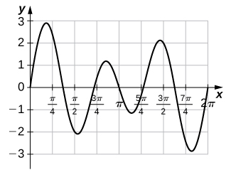
65) [T] The following graph is of a function of the form \(\displaystylef(t)=asin(nt)+bsin(mt)\). Estimate the coefficients a and b, and the frequency parameters n and m. Use these estimates to approximate \(\displaystyle∫^π_0f(t)dt\).

66) [T] The following graph is of a function of the form \(\displaystylef(x)=acos(nt)+bcos(mt)\). Estimate the coefficients a and b and the frequency parameters n and m. Use these estimates to approximate \(\displaystyle∫^π_0f(t)dt.\)

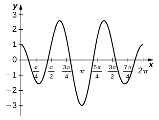
Solution: \(\displaystylef(t)=2cos(3t)−cos(2t);∫^{π/2}_0(2cos(3t)−cos(2t))=−\frac{2}{3}\)

5.6: Integrals Involving Exponential and Logarithmic Functions

In the following exercises, compute each indefinite integral.

1) \(\displaystyle ∫e^{2x}dx\)

2) \(\displaystyle ∫e^{−3x}dx\)

Solution: \(\displaystyle \frac{−1}{3}e^{−3x}+C\)

3) \(\displaystyle ∫2^xdx\)

4) \(\displaystyle ∫3^{−x}dx\)

Solution: \(\displaystyle −\frac{3^{−x}}{ln3}+C\)

5) \(\displaystyle ∫\frac{1}{2x}dx\)

6) \(\displaystyle ∫\frac{2}{x}dx\)

Solution: \(\displaystyle ln(x^2)+C\)

7) \(\displaystyle ∫\frac{1}{x^2}dx\)

8) \(\displaystyle ∫\frac{1}{\sqrt{x}}dx\)

Soltuion: \(\displaystyle 2\sqrt{x}+C\)

In the following exercises, find each indefinite integral by using appropriate substitutions.

9) \(\displaystyle ∫\frac{lnx}{x}dx\)

10) \(\displaystyle ∫\frac{dx}{x(lnx)^2}\)

Solution: \(\displaystyle −\frac{1}{lnx}+C\)

11) \(\displaystyle ∫\frac{dx}{xlnx}(x>1)\)

12) \(\displaystyle ∫\frac{dx}{xlnxln(lnx)}\)

Solution: \(\displaystyle ln(ln(lnx))+C\)

13) \(\displaystyle ∫tanθdθ\)

14) \(\displaystyle ∫\frac{cosx−xsinx}{xcosx}dx\)

Solution: \(\displaystyle ln(xcosx)+C\)

15) \(\displaystyle ∫\frac{ln(sinx)}{tanx}dx\)

16) \(\displaystyle ∫ln(cosx)tanxdx\)

Solution: \(\displaystyle −\frac{1}{2}(ln(cos(x)))^2+C\)

17) \(\displaystyle ∫xe^{−x^2}dx\)

18) \(\displaystyle ∫x^2e^{−x^3}dx\)

Solution: \(\displaystyle \frac{−e^{−x^3}}{3}+C\)

19) \(\displaystyle ∫e^{sinx}cosxdx\)

20) \(\displaystyle ∫e^{tanx}sec^2xdx\)

Solution: \(\displaystyle e^{tanx}+C\)

21) \(\displaystyle ∫e^{lnx}\frac{dx}{x}\)

22) \(\displaystyle ∫\frac{e^{ln(1−t)}}{1−t}dt\)

Solution: \(\displaystyle t+C\)

In the following exercises, verify by differentiation that \(\displaystyle ∫lnxdx=x(lnx−1)+C\), then use appropriate changes of variables to compute the integral.

23) \(\displaystyle ∫lnxdx (Hint:∫lnxdx=\frac{1}{2}∫xln(x^2)dx)\)

24) \(\displaystyle ∫x^2ln^2xdx\)

Solution: \(\displaystyle \frac{1}{9}x^3(ln(x^3)−1)+C\)

25) \(\displaystyle ∫\frac{lnx}{x^2}dx\) (Hint:Set \(\displaystyle u=\frac{1}{x}.)\)

26) \(\displaystyle ∫\frac{lnx}{\sqrt{x}}dx\) (Hint:Set \(\displaystyle u=\sqrt{x}.)\)

Solution: \(\displaystyle 2\sqrt{x}(lnx−2)+C\)

27) Write an integral to express the area under the graph of \(\displaystyle y=\frac{1}{t}\) from \(\displaystyle t=1\) to \(\displaystyle e^x\) and evaluate the integral.

28) Write an integral to express the area under the graph of \(\displaystyle y=e^t\) between \(\displaystyle t=0\) and \(\displaystyle t=lnx\), and evaluate the integral.

Solution: \(\displaystyle ∫^{lnx}_0e^tdt=e^t∣^{lnx}_0=e^{lnx}−e^0=x−1\)

In the following exercises, use appropriate substitutions to express the trigonometric integrals in terms of compositions with logarithms.

29) \(\displaystyle ∫tan(2x)dx\)

30) \(\displaystyle ∫\frac{sin(3x)−cos(3x)}{sin(3x)+cos(3x)}dx\)

Solution: \(\displaystyle −\frac{1}{3}ln(sin(3x)+cos(3x))\)

31) \(\displaystyle ∫\frac{xsin(x^2)}{cos(x^2)}dx\)

32) \(\displaystyle ∫xcsc(x^2)dx\)

Solution: \(\displaystyle −\frac{1}{2}ln∣csc(x^2)+cot(x^2)∣+C\)

33) \(\displaystyle ∫ln(cosx)tanxdx\)

34) \(\displaystyle ∫ln(cscx)cotxdx\)

Solution: \(\displaystyle −\frac{1}{2}(ln(cscx))^2+C\)

35) \(\displaystyle ∫\frac{e^x−e^{−x}}{e^x+e^{−x}}dx\)

In the following exercises, evaluate the definite integral.

36) \(\displaystyle ∫^2_1\frac{1+2x+x^2}{3x+3x^2+x^3}dx\)

Solution: \(\displaystyle \frac{1}{3}ln(\frac{26}{7})\)

37) \(\displaystyle ∫^{π/4}_0tanxdx\)

38) \(\displaystyle ∫^{π/3}_0\frac{sinx−cosx}{sinx+cosx}dx\)

Solutnio: \(\displaystyle ln(\sqrt{3}−1)\)

39) \(\displaystyle ∫^{π/2}_{π/6}cscxdx\)

40) \(\displaystyle ∫^{π/3}_{π/4}cotxdx\)

Solution: \(\displaystyle \frac{1}{2}ln\frac{3}{2}\)

In the following exercises, integrate using the indicated substitution.

41) \(\displaystyle ∫\frac{x}{x−100}dx;u=x−100\)

42) \(\displaystyle ∫\frac{y−1}{y+1}dy;u=y+1\)

Solution: \(\displaystyle y−2ln|y+1|+C\)

43) \(\displaystyle ∫\frac{1−x^2}{3x−x^3}dx;u=3x−x^3\)

44) \(\displaystyle ∫\frac{sinx+cosx}{sinx−cosx}dx;u=sinx−cosx\)

Solution: \(\displaystyle ln|sinx−cosx|+C\)

45) \(\displaystyle ∫e^{2x}\sqrt{1−e^{2x}}dx;u=e^{2x}\)

46) \(\displaystyle ∫ln(x)\frac{\sqrt{1−(lnx)^2}}{x}dx;u=lnx\)

Solution: \(\displaystyle −\frac{1}{3}(1−(lnx^2))^{3/2}+C\)

In the following exercises, does the right-endpoint approximation overestimate or underestimate the exact area? Calculate the right endpoint estimate R₅₀ and solve for the exact area.

47) [T] \(\displaystyle y=e^x\) over \(\displaystyle [0,1]\)

48) [T] \(\displaystyle y=e^{−x}\) over \(\displaystyle [0,1]\)

Solution: Exact solution: \(\displaystyle \frac{e−1}{e},R_{50}=0.6258\). Since f is decreasing, the right endpoint estimate underestimates the area.

49) [T] \(\displaystyle y=ln(x)\) over \(\displaystyle [1,2]\)

50) [T] \(\displaystyle y=\frac{x+1}{x^2+2x+6}\) over \(\displaystyle [0,1]\)

Solution: Exact solution: \(\displaystyle \frac{2ln(3)−ln(6)}{2},R_{50}=0.2033.\) Since f is increasing, the right endpoint estimate overestimates the area.

51) [T] \(\displaystyle y=2^x\) over \(\displaystyle [−1,0]\)

52) [T] \(\displaystyle y=−2^{−x}\)over \(\displaystyle [0,1]\)

Solution: Exact solution: \(\displaystyle −\frac{1}{ln(4)},R_{50}=−0.7164.\) Since f is increasing, the right endpoint estimate overestimates the area (the actual area is a larger negative number).

In the following exercises, \(\displaystyle f(x)≥0\) for \(\displaystyle a≤x≤b\). Find the area under the graph of \(\displaystyle f(x)\) between the given values a and b by integrating.

53) \(\displaystyle f(x)=\frac{log_{10}(x)}{x};a=10,b=100\)

54) \(\displaystyle f(x)=\frac{log_2(x)}{x};a=32,b=64\)

Solution: \(\displaystyle \frac{11}{2}ln2\)

55) \(\displaystyle f(x)=2^{−x};a=1,b=2\)

56) \(\displaystyle f(x)=2^{−x};a=3,b=4\)

Solution: \(\displaystyle \frac{1}{ln(65,536)}\)

57) Find the area under the graph of the function \(\displaystyle f(x)=xe^{−x^2}\) between \(\displaystyle x=0\) and \(\displaystyle x=5\).

58) Compute the integral of \(\displaystyle f(x)=xe^{−x^2}\) and find the smallest value of N such that the area under the graph \(\displaystyle f(x)=xe^{−x^2}\) between \(\displaystyle x=N\) and \(\displaystyle x=N+10\) is, at most, 0.01.

Solution: \(\displaystyle ∫^{N+1}_Nxe^{−x^2}dx=\frac{1}{2}(e^{−N^2}−e^{−(N+1)^2}).\) The quantity is less than 0.01 when \(\displaystyle N=2\).

59) Find the limit, as N tends to infinity, of the area under the graph of \(\displaystyle f(x)=xe^{−x^2}\) between \(\displaystyle x=0\) and \(\displaystyle x=5\).

60) Show that \(\displaystyle ∫^b_a\frac{dt}{t}=∫^{1/a}_{1/b}\frac{dt}{t}\) when \(\displaystyle 0<a≤b\).

Solution: \(\displaystyle ∫^b_a\frac{dx}{x}=ln(b)−ln(a)=ln(\frac{1}{a})−ln(\frac{1}{b})=∫^{1/a}_{1/b}\frac{dx}{x}\)

61) Suppose that \(\displaystyle f(x)>0\) for all x and that f and g are differentiable. Use the identity \(\displaystyle f^g=e^{glnf}\) and the chain rule to find the derivative of \(\displaystyle f^g\).

62) Use the previous exercise to find the antiderivative of \(\displaystyle h(x)=x^x(1+lnx)\) and evaluate \(\displaystyle ∫^3_2x^x(1+lnx)dx\).

Solution: 23

63) Show that if \(\displaystyle c>0\), then the integral of \(\displaystyle 1/x\) from ac to bc \(\displaystyle (0<a<b)\) is the same as the integral of \(\displaystyle 1/x\) from a to b.

The following exercises are intended to derive the fundamental properties of the natural log starting from the definition \(\displaystyle ln(x)=∫^x_1\frac{dt}{t}\), using properties of the definite integral and making no further assumptions.

64) Use the identity \(\displaystyle ln(x)=∫^x_1\frac{dt}{t}\) to derive the identity \(\displaystyle ln(\frac{1}{x})=−lnx\).

Solution: We may assume that \(\displaystyle x>1\),so \(\displaystyle \frac{1}{x}<1.\) Then, \(\displaystyle ∫^{1/x}_{1}\frac{dt}{t}\). Now make the substitution \(\displaystyle u=\frac{1}{t}\), so \(\displaystyle du=−\frac{dt}{t^2}\) and \(\displaystyle \frac{du}{u}=−\frac{dt}{t}\), and change endpoints: \(\displaystyle ∫^{1/x}_1\frac{dt}{t}=−∫^x_1\frac{du}{u}=−lnx.\)

65) Use a change of variable in the integral \(\displaystyle ∫^{xy}_1\frac{1}{t}dt\) to show that \(\displaystyle lnxy=lnx+lny\) for \(\displaystyle x,y>0\).

66) Use the identity \(\displaystyle lnx=∫^x_1\frac{dt}{x}\) to show that \(\displaystyle ln(x)\) is an increasing function of x on \(\displaystyle [0,∞)\), and use the previous exercises to show that the range of \(\displaystyle ln(x)\) is \(\displaystyle (−∞,∞)\). Without any further assumptions, conclude that \(\displaystyle ln(x)\) has an inverse function defined on \(\displaystyle (−∞,∞).\)

67) Pretend, for the moment, that we do not know that \(\displaystyle e^x\) is the inverse function of \(\displaystyle ln(x)\), but keep in mind that \(\displaystyle ln(x)\) has an inverse function defined on \(\displaystyle (−∞,∞)\). Call it E. Use the identity \(\displaystyle lnxy=lnx+lny\) to deduce that \(\displaystyle E(a+b)=E(a)E(b)\) for any real numbers a, b.

68) Pretend, for the moment, that we do not know that \(\displaystyle e^x\) is the inverse function of \(\displaystyle lnx\), but keep in mind that \(\displaystyle lnx\) has an inverse function defined on \(\displaystyle (−∞,∞)\). Call it E. Show that \(\displaystyle E'(t)=E(t).\)

Solution: \(\displaystyle x=E(ln(x)).\) Then, \(\displaystyle 1=\frac{E'(lnx)}{x}\) or \(\displaystyle x=E'(lnx)\). Since any number t can be written \(\displaystyle t=lnx\) for some x, and for such t we have \(\displaystyle x=E(t)\), it follows that for any \(\displaystyle t,E'(t)=E(t).\)

69) The sine integral, defined as \(\displaystyle S(x)=∫^x_0\frac{sint}{t}dt\) is an important quantity in engineering. Although it does not have a simple closed formula, it is possible to estimate its behavior for large x. Show that for \(\displaystyle k≥1,|S(2πk)−S(2π(k+1))|≤\frac{1}{k(2k+1)π}.\) (Hint: \(\displaystyle sin(t+π)=−sint\))

70) [T] The normal distribution in probability is given by \(\displaystyle p(x)=\frac{1}{σ\sqrt{2π}}e^{−(x−μ)^2/2σ^2}\), where σ is the standard deviation and μ is the average. The standard normal distribution in probability, \(\displaystyle p_s\), corresponds to \(\displaystyle μ=0\) and \(\displaystyle σ=1\). Compute the left endpoint estimates \(\displaystyle R_{10}\) and \(\displaystyle R_{100}\) of \(\displaystyle ∫^1_{−1}\frac{1}{\sqrt{2π}}e^{−x^{2/2}}dx.\)

Solution: \(\displaystyle R_{10}=0.6811,R_{100}=0.6827\)

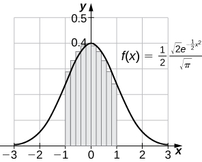
71) [T] Compute the right endpoint estimates \(\displaystyle R_{50}\) and \(\displaystyle R_{100}\) of \(\displaystyle ∫^5_{−3}\frac{1}{2\sqrt{2π}}e^{−(x−1)^2/8}\).

5.7: Integrals Resulting in Inverse Trigonometric Functions

In the following exercises, evaluate each integral in terms of an inverse trigonometric function.

1) \(\displaystyle ∫^{\sqrt{3}/2}_0\frac{dx}{\sqrt{1−x^2}}\)

Solution: \(\displaystyle sin^{−1}x∣^{\sqrt{3}/2}_0=\frac{π}{3}\)

2) \(\displaystyle ∫^{1/2}_{−1/2}\frac{dx}{\sqrt{1−x^2}}\)

3) \(\displaystyle ∫^1_{\sqrt{3}}\frac{dx}{\sqrt{1+x^2}}\)

Solution: \(\displaystyle tan^{−1}x∣^1_{\sqrt{3}}=−\frac{π}{12}\)

4) \(\displaystyle ∫^{\sqrt{3}}_{\frac{1}{\sqrt{3}}}\frac{dx}{1+x^2}\)

5) \(\displaystyle ∫^{\sqrt{2}}_1\frac{dx}{|x|\sqrt{x^2−1}}\)

Solution: \(\displaystyle sec^{−1}x∣^{\sqrt{2}}_1=\frac{π}{4}\)

6) \(\displaystyle ∫^{\frac{2}{\sqrt{3}}}_1\frac{dx}{|x|\sqrt{x^2−1}}\)

In the following exercises, find each indefinite integral, using appropriate substitutions.

7) \(\displaystyle ∫\frac{dx}{\sqrt{9−x^2}}\)

Solution: \(\displaystyle sin^{−1}(\frac{x}{3})+C\)

8) \(\displaystyle ∫\frac{dx}{\sqrt{1−16x^2}}\)

9) \(\displaystyle ∫\frac{dx}{9+x^2}\)

Solution: \(\displaystyle \frac{1}{3}tan^{−1}(\frac{x}{3})+C\)

10) \(\displaystyle ∫\frac{dx}{25+16x^2}\)

11) \(\displaystyle ∫\frac{dx}{|x|\sqrt{x^2−9}}\)

Solution: \(\displaystyle \frac{1}{3}sec^{−1}(\frac{x}{3})+C\)

12) \(\displaystyle ∫\frac{dx}{|x|\sqrt{4x^2−16}}\)

13) Explain the relationship \(\displaystyle −cos^{−}1t+C=∫\frac{dt}{\sqrt{1−t^2}}=sin^{−1}t+C.\) Is it true, in general, that \(\displaystyle cos^{−1}t=−sin^{−1}t\)?

Solution: \(\displaystyle cos(\frac{π}{2}−θ)=sinθ.\) So, \(\displaystyle sin^{−1}t=\frac{π}{2}−cos^{−1}t.\) They differ by a constant.

14) Explain the relationship \(\displaystyle sec^{−1}t+C=∫\frac{dt}{|t|sqrt{t^2−1}}=−csc^{−1}t+C.\) Is it true, in general, that \(\displaystyle sec^{−1}t=−csc^{−1}t\)?

15) Explain what is wrong with the following integral: \(\displaystyle ∫^2_1\frac{dt}{\sqrt{1−t^2}}\).

Soution: \(\displaystyle \sqrt{1−t^2}\) is not defined as a real number when \(\displaystyle t>1\).

16) Explain what is wrong with the following integral: \(\displaystyle ∫^1_{−1}\frac{dt}{|t|\sqrt{t^2−1}}\).

In the following exercises, solve for the antiderivative \(\displaystyle ∫f\) of f with \(\displaystyle C=0\), then use a calculator to graph f and the antiderivative over the given interval \(\displaystyle [a,b]\). Identify a value of C such that adding C to the antiderivative recovers the definite integral \(\displaystyle F(x)=∫^x_af(t)dt\).

17) [T] \(\displaystyle ∫\frac{1}{\sqrt{9−x^2}}dx\) over \(\displaystyle [−3,3]\)

Solution:

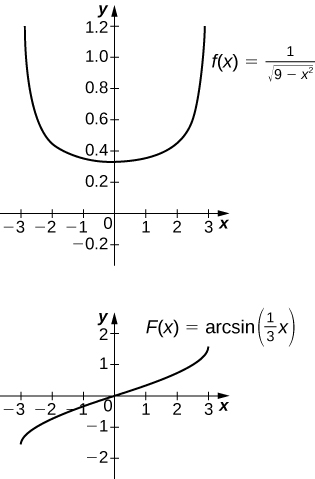
The antiderivative is \(\displaystyle sin^{−1}(\frac{x}{3})+C\). Taking \(\displaystyle C=\frac{π}{2}\) recovers the definite integral.

18) [T] \(\displaystyle ∫\frac{9}{9+x^2}dx\) over \(\displaystyle [−6,6]\)

19) [T] \(\displaystyle ∫\frac{cosx}{4+sin^2x}dx\) over \(\displaystyle [−6,6]\)

Solution:

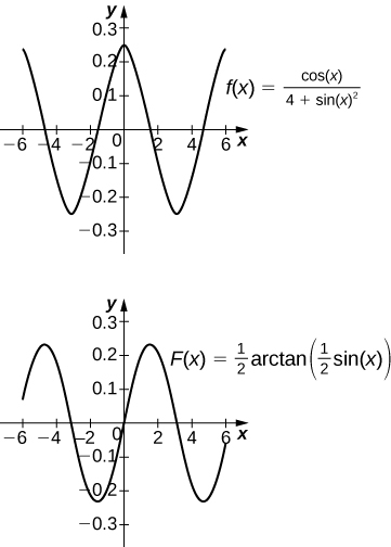
The antiderivative is \(\displaystyle \frac{1}{2}tan^{−1}(\frac{sinx}{2})+C\). Taking \(\displaystyle C=\frac{1}{2}tan^{−1}(\frac{sin(6)}{2})\) recovers the definite integral.

20) [T] \(\displaystyle ∫\frac{e^x}{1+e^{2x}}dx\) over \(\displaystyle [−6,6]\)

In the following exercises, compute the antiderivative using appropriate substitutions.

21) \(\displaystyle ∫\frac{sin^{−1}tdt}{\sqrt{1−t^2}}\)

Solution: \(\displaystyle \frac{1}{2}(sin^{−1}t)^2+C\)

22) \(\displaystyle ∫\frac{dt}{sin^{−1}\sqrt{t^1−t^2}}\)

23) \(\displaystyle ∫\frac{tan^{−1}(2t)1}+4t^2dt\)

Soluion: \frac{1}{4}(tan^{−1}(2t))^2\)

24\) ∫\frac{ttan^{−1}{t^2}1+t4dt

25) \(\displaystyle ∫sec^{−1}\frac{(}{t}2)|t|\sqrt{t^2−4}dt\)

Solution:L \(\displaystyle \frac{1}{4}(sec^{−1}(\frac{t}{2})2)+\)

26) \(\displaystyle ∫\frac{tsec^{−1}(t^2)}{t^2\sqrt{t^4−1}}dt\)

In the following exercises, use a calculator to graph the antiderivative \(\displaystyle ∫f\) with \(\displaystyle C=0\) over the given interval \(\displaystyle [a,b].\) Approximate a value of C, if possible, such that adding C to the antiderivative gives the same value as the definite integral \(\displaystyle F(x)=∫^x_af(t)dt.\)

27) [T] \(\displaystyle ∫\frac{1}{x\sqrt{x^2−4}}dx\) over \(\displaystyle [2,6]\)

Solution:

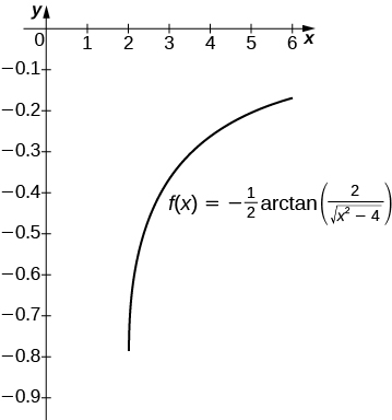
The antiderivative is \(\displaystyle \frac{1}{2}sec^{−1}(\frac{x}{2})+C\). Taking \(\displaystyle C=0\) recovers the definite integral over \(\displaystyle [2,6]\).

28) [T] \(\displaystyle ∫\frac{1}{(2x+2)\sqrt{x}}dx\) over \(\displaystyle [0,6]\)

29) [T] \(\displaystyle ∫\frac{(sinx+xcosx)}{1+x^2sin^2xdx}\) over \(\displaystyle [−6,6]\)

Solution:

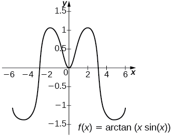
The general antiderivative is \(\displaystyle tan^{−1}(xsinx)+C\). Taking \(\displaystyle C=−tan^{−1}(6sin(6))\) recovers the definite integral.

30) [T] \(\displaystyle ∫\frac{2e^{−2x}}{\sqrt{1−e^{−4x}}}dx\) over \(\displaystyle [0,2]\)

31) [T] \(\displaystyle ∫\frac{1}{x+xln2x}\) over \(\displaystyle [0,2]\)

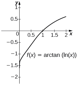
The general antiderivative is \(\displaystyle tan^{−1}(lnx)+C\). Taking \(\displaystyle C=\frac{π}{2}=tan^{−1}∞\) recovers the definite integral.

32) [T] \(\displaystyle ∫\frac{sin^{−1}x}{\sqrt{1−x^2}}\) over \(\displaystyle [−1,1]\)

In the following exercises, compute each integral using appropriate substitutions.

33) \(\displaystyle ∫\frac{e^x}{\sqrt{1−e^{2t}}}dt\)

Solutnio: \(\displaystyle sin^{−1}(e^t)+C\)

34) \(\displaystyle ∫\frac{e^t}{1+e^{2t}}dt\)

35) \(\displaystyle ∫\frac{dt}{t\sqrt{1−ln^2t}}\)

Solution: \(\displaystyle sin^{−1}(lnt)+C\)

36) \(\displaystyle ∫\frac{dt}{t(1+ln^2t)}\)

37) \(\displaystyle ∫\frac{cos^{−1}(2t)}{\sqrt{1−4t^2}}dt\)

Solution: \(\displaystyle −\frac{1}{2}(cos^{−1}(2t))^2+C\)

38) \(\displaystyle ∫\frac{e^tcos^{−1}(e^t)}{\sqrt{1−e^{2t}}}dt\)

In the following exercises, compute each definite integral.

39) \(\displaystyle ∫^{1/2}|_0\frac{tan(sin^{−1}t)}{\sqrt{1−t^2}}dt\)

Solution: \(\displaystyle \frac{1}{2}ln(\frac{4}{3})\)

40) \(\displaystyle ∫^{1/2}_{1/4}\frac{tan(cos^{−1}t)}{\sqrt{1−t^2}}dt\)

41) \(\displaystyle ∫^{1/2}_0\frac{sin(tan^{−1}t)}{1+t^2}dt\)

Solution: \(\displaystyle 1−\frac{2}{\sqrt{5}}\)

42) \(\displaystyle ∫^{1/2}_0\frac{cos(tan^{−1}t)}{1+t^2}dt\0

43) For \(\displaystyle A>0\), compute \(\displaystyle I(A)=∫^{A}_{−A}\frac{dt}{1+t^2}\) and evaluate \(\displaystyle \lim_{a→∞}I(A)\), the area under the graph of \(\displaystyle \frac{1}{1+t^2}\) on \(\displaystyle [−∞,∞]\).

Solution: \(\displaystyle 2tan^{−1}(A)→π\) as \(\displaystyle A→∞\)

44) For \(\displaystyle 1<B<∞\), compute \(\displaystyle I(B)=∫^B_1\frac{dt}{t\sqrt{t^2−1}}\) and evaluate \(\displaystyle \lim_{B→∞}I(B)\), the area under the graph of \(\displaystyle \frac{1}{t\sqrt{t^2−1}}\) over \(\displaystyle [1,∞)\).

45) Use the substitution \(\displaystyle u=\sqrt{2}cotx\) and the identity 1 \(\displaystyle +cot^2x=csc^2x\) to evaluate \(\displaystyle ∫\frac{dx}{1+cos^2x}\). (Hint: Multiply the top and bottom of the integrand by \(\displaystyle csc^2x\).)

Solution: Using the hint, one has \(\displaystyle ∫\frac{csc^2x}{csc^2x+cot^2x}dx=∫\frac{csc^2x}{1+2cot^2x}dx.\) Set \(\displaystyle u=\sqrt{2}cotx.\) Then, \(\displaystyle du=−\sqrt{2}csc^2x\) and the integral is \(\displaystyle −\frac{1}{\sqrt{2}}∫\frac{du}{1+u^2}=−\frac{1}{\sqrt{2}}tan^{−1}u+C=\frac{1}{\sqrt{2}}tan^{−1}(\sqrt{2}cotx)+C\). If one uses the identity \(\displaystyle tan^{−1}s+tan^{−1}(\frac{1}{s})=\frac{π}{2}\), then this can also be written \(\displaystyle \frac{1}{\sqrt{2}}tan^{−1}(\frac{tanx}{\sqrt{2}})+C.\)

46) [T] Approximate the points at which the graphs of \(\displaystyle f(x)=2x^2−1\) and \(\displaystyle g(x)=(1+4x^2)^{−3/2}\) intersect, and approximate the area between their graphs accurate to three decimal places.

47) [T] Approximate the points at which the graphs of \(\displaystyle f(x)=x^2−1\) and \(\displaystyle f(x)=x^2−1\) intersect, and approximate the area between their graphs accurate to three decimal places.

Solution: \(\displaystyle x≈±1.13525.\) The left endpoint estimate with \(\displaystyle N=100\) is 2.796 and these decimals persist for \(\displaystyle N=500\).

48) Use the following graph to prove that \(\displaystyle ∫^x_0\sqrt{1−t^2}dt=\frac{1}{2}x\sqrt{1−x^2}+\frac{1}{2}sin^{−1}x.\)

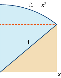
Chapter Review Exercises:

True or False. Justify your answer with a proof or a counterexample. Assume all functions \(\displaystyle f\) and \(\displaystyle g\) are continuous over their domains.

1) If \(\displaystyle f(x)>0,f′(x)>0\) for all \(\displaystyle x\), then the right-hand rule underestimates the integral \(\displaystyle ∫^b_af(x).\) Use a graph to justify your answer.

Solution: False

2) \(\displaystyle ∫^b_af(x)^2dx=∫^b_af(x)dx∫^b_af(x)dx\)

3) If \(\displaystyle f(x)≤g(x)\) for all \(\displaystyle x∈[a,b]\), then \(\displaystyle ∫^b_af(x)≤∫^b_ag(x).\)

Solution: True

4) All continuous functions have an antiderivative.

Evaluate the Riemann sums \(\displaystyle L_4\) and \(\displaystyle R_4\) for the following functions over the specified interval. Compare your answer with the exact answer, when possible, or use a calculator to determine the answer.

5) \(\displaystyle y=3x^2−2x+1)\) over \(\displaystyle [−1,1]\)

Solution: \(\displaystyle L_4=5.25,R_4=3.25,\) exact answer: 4

6) \(\displaystyle y=ln(x^2+1)\) over \(\displaystyle [0,e]\)

7) \(\displaystyle y=x^2sinx\) over \(\displaystyle [0,π]\)

Solution: \(\displaystyle L_4=5.364,R_4=5.364,\) exact answer: \(\displaystyle 5.870\)

8) \(\displaystyle y=\sqrt{x}+\frac{1}{x}\) over \(\displaystyle [1,4]\)

Evaluate the following integrals.

9) \(\displaystyle ∫^1_{−1}(x^3−2x^2+4x)dx\)

Solution: \(\displaystyle −\frac{4}{3}\)

10) \(\displaystyle ∫^4_0\frac{3t}{\sqrt{1+6t^2}}dt\)

11) \(\displaystyle ∫^{π/2}_{π/3}2sec(2θ)tan(2θ)dθ\)

Solution: 1

12) \(\displaystyle ∫^{π/4}_0e^{cos^2x}sinxcosdx\)

Find the antiderivative.

13) \(\displaystyle ∫\frac{dx}{(x+4)^3}\)

Solution: \(\displaystyle −\frac{1}{2(x+4)^2}+C\)

14) \(\displaystyle ∫xln(x^2)dx\)

15) \(\displaystyle ∫\frac{4x^2}{\sqrt{1−x^6}}dx\)

Solution: \(\displaystyle \frac{4}{3}sin^{−1}(x^3)+C\)

16) \(\displaystyle ∫\frac{e^{2x}}{1+e^{4x}}dx\)

Find the derivative.

17) \(\displaystyle \frac{d}{dt}∫^t_0\frac{sinx}{\sqrt{1+x^2}}dx\)

Solution: \(\displaystyle \frac{sint}{\sqrt{1+t^2}}\)

18) \(\displaystyle \frac{d}{dx}∫^{x^3}_1\sqrt{4−t^2}dt\)

19) \(\displaystyle \frac{d}{dx}∫^{ln(x)}_1(4t+e^t)dt\)

Solution: \(\displaystyle 4\frac{lnx}{x}+1\)

20) \(\displaystyle \frac{d}{dx}∫^{cosx}_0e^{t^2}dt\)

The following problems consider the historic average cost per gigabyte of RAM on a computer.

Year	5-Year Change ($)
1980	0
1985	−5,468,750
1990	−755,495
1995	−73,005
2000	−29,768
2005	−918
2010	−177

21) If the average cost per gigabyte of RAM in 2010 is $12, find the average cost per gigabyte of RAM in 1980.

Solution: $6,328,113

22) The average cost per gigabyte of RAM can be approximated by the function \(\displaystyle C(t)=8,500,000(0.65)^t\), where \(\displaystyle t\) is measured in years since 1980, and \(\displaystyle C\) is cost in US$. Find the average cost per gigabyte of RAM for 1980 to 2010.

23) Find the average cost of 1GB RAM for 2005 to 2010.

Solution: $73.36

24) The velocity of a bullet from a rifle can be approximated by \(\displaystyle v(t)=6400t^2−6505t+2686,\) where \(\displaystyle t\) is seconds after the shot and v is the velocity measured in feet per second. This equation only models the velocity for the first half-second after the shot: \(\displaystyle 0≤t≤0.5.\) What is the total distance the bullet travels in 0.5 sec?

25) What is the average velocity of the bullet for the first half-second?

Solution: \(\displaystyle \frac{19117}{12}ft/sec,or1593ft/sec\)