
4.1: Solving Linear Systems by Graphing
- Page ID
- 18347
\( \newcommand{\vecs}[1]{\overset { \scriptstyle \rightharpoonup} {\mathbf{#1}} } \)
\( \newcommand{\vecd}[1]{\overset{-\!-\!\rightharpoonup}{\vphantom{a}\smash {#1}}} \)
\( \newcommand{\dsum}{\displaystyle\sum\limits} \)
\( \newcommand{\dint}{\displaystyle\int\limits} \)
\( \newcommand{\dlim}{\displaystyle\lim\limits} \)
\( \newcommand{\id}{\mathrm{id}}\) \( \newcommand{\Span}{\mathrm{span}}\)
( \newcommand{\kernel}{\mathrm{null}\,}\) \( \newcommand{\range}{\mathrm{range}\,}\)
\( \newcommand{\RealPart}{\mathrm{Re}}\) \( \newcommand{\ImaginaryPart}{\mathrm{Im}}\)
\( \newcommand{\Argument}{\mathrm{Arg}}\) \( \newcommand{\norm}[1]{\| #1 \|}\)
\( \newcommand{\inner}[2]{\langle #1, #2 \rangle}\)
\( \newcommand{\Span}{\mathrm{span}}\)
\( \newcommand{\id}{\mathrm{id}}\)
\( \newcommand{\Span}{\mathrm{span}}\)
\( \newcommand{\kernel}{\mathrm{null}\,}\)
\( \newcommand{\range}{\mathrm{range}\,}\)
\( \newcommand{\RealPart}{\mathrm{Re}}\)
\( \newcommand{\ImaginaryPart}{\mathrm{Im}}\)
\( \newcommand{\Argument}{\mathrm{Arg}}\)
\( \newcommand{\norm}[1]{\| #1 \|}\)
\( \newcommand{\inner}[2]{\langle #1, #2 \rangle}\)
\( \newcommand{\Span}{\mathrm{span}}\) \( \newcommand{\AA}{\unicode[.8,0]{x212B}}\)
\( \newcommand{\vectorA}[1]{\vec{#1}} % arrow\)
\( \newcommand{\vectorAt}[1]{\vec{\text{#1}}} % arrow\)
\( \newcommand{\vectorB}[1]{\overset { \scriptstyle \rightharpoonup} {\mathbf{#1}} } \)
\( \newcommand{\vectorC}[1]{\textbf{#1}} \)
\( \newcommand{\vectorD}[1]{\overrightarrow{#1}} \)
\( \newcommand{\vectorDt}[1]{\overrightarrow{\text{#1}}} \)
\( \newcommand{\vectE}[1]{\overset{-\!-\!\rightharpoonup}{\vphantom{a}\smash{\mathbf {#1}}}} \)
\( \newcommand{\vecs}[1]{\overset { \scriptstyle \rightharpoonup} {\mathbf{#1}} } \)
\(\newcommand{\longvect}{\overrightarrow}\)
\( \newcommand{\vecd}[1]{\overset{-\!-\!\rightharpoonup}{\vphantom{a}\smash {#1}}} \)
\(\newcommand{\avec}{\mathbf a}\) \(\newcommand{\bvec}{\mathbf b}\) \(\newcommand{\cvec}{\mathbf c}\) \(\newcommand{\dvec}{\mathbf d}\) \(\newcommand{\dtil}{\widetilde{\mathbf d}}\) \(\newcommand{\evec}{\mathbf e}\) \(\newcommand{\fvec}{\mathbf f}\) \(\newcommand{\nvec}{\mathbf n}\) \(\newcommand{\pvec}{\mathbf p}\) \(\newcommand{\qvec}{\mathbf q}\) \(\newcommand{\svec}{\mathbf s}\) \(\newcommand{\tvec}{\mathbf t}\) \(\newcommand{\uvec}{\mathbf u}\) \(\newcommand{\vvec}{\mathbf v}\) \(\newcommand{\wvec}{\mathbf w}\) \(\newcommand{\xvec}{\mathbf x}\) \(\newcommand{\yvec}{\mathbf y}\) \(\newcommand{\zvec}{\mathbf z}\) \(\newcommand{\rvec}{\mathbf r}\) \(\newcommand{\mvec}{\mathbf m}\) \(\newcommand{\zerovec}{\mathbf 0}\) \(\newcommand{\onevec}{\mathbf 1}\) \(\newcommand{\real}{\mathbb R}\) \(\newcommand{\twovec}[2]{\left[\begin{array}{r}#1 \\ #2 \end{array}\right]}\) \(\newcommand{\ctwovec}[2]{\left[\begin{array}{c}#1 \\ #2 \end{array}\right]}\) \(\newcommand{\threevec}[3]{\left[\begin{array}{r}#1 \\ #2 \\ #3 \end{array}\right]}\) \(\newcommand{\cthreevec}[3]{\left[\begin{array}{c}#1 \\ #2 \\ #3 \end{array}\right]}\) \(\newcommand{\fourvec}[4]{\left[\begin{array}{r}#1 \\ #2 \\ #3 \\ #4 \end{array}\right]}\) \(\newcommand{\cfourvec}[4]{\left[\begin{array}{c}#1 \\ #2 \\ #3 \\ #4 \end{array}\right]}\) \(\newcommand{\fivevec}[5]{\left[\begin{array}{r}#1 \\ #2 \\ #3 \\ #4 \\ #5 \\ \end{array}\right]}\) \(\newcommand{\cfivevec}[5]{\left[\begin{array}{c}#1 \\ #2 \\ #3 \\ #4 \\ #5 \\ \end{array}\right]}\) \(\newcommand{\mattwo}[4]{\left[\begin{array}{rr}#1 \amp #2 \\ #3 \amp #4 \\ \end{array}\right]}\) \(\newcommand{\laspan}[1]{\text{Span}\{#1\}}\) \(\newcommand{\bcal}{\cal B}\) \(\newcommand{\ccal}{\cal C}\) \(\newcommand{\scal}{\cal S}\) \(\newcommand{\wcal}{\cal W}\) \(\newcommand{\ecal}{\cal E}\) \(\newcommand{\coords}[2]{\left\{#1\right\}_{#2}}\) \(\newcommand{\gray}[1]{\color{gray}{#1}}\) \(\newcommand{\lgray}[1]{\color{lightgray}{#1}}\) \(\newcommand{\rank}{\operatorname{rank}}\) \(\newcommand{\row}{\text{Row}}\) \(\newcommand{\col}{\text{Col}}\) \(\renewcommand{\row}{\text{Row}}\) \(\newcommand{\nul}{\text{Nul}}\) \(\newcommand{\var}{\text{Var}}\) \(\newcommand{\corr}{\text{corr}}\) \(\newcommand{\len}[1]{\left|#1\right|}\) \(\newcommand{\bbar}{\overline{\bvec}}\) \(\newcommand{\bhat}{\widehat{\bvec}}\) \(\newcommand{\bperp}{\bvec^\perp}\) \(\newcommand{\xhat}{\widehat{\xvec}}\) \(\newcommand{\vhat}{\widehat{\vvec}}\) \(\newcommand{\uhat}{\widehat{\uvec}}\) \(\newcommand{\what}{\widehat{\wvec}}\) \(\newcommand{\Sighat}{\widehat{\Sigma}}\) \(\newcommand{\lt}{<}\) \(\newcommand{\gt}{>}\) \(\newcommand{\amp}{&}\) \(\definecolor{fillinmathshade}{gray}{0.9}\)- Check solutions to systems of linear equations.
- Solve linear systems using the graphing method.
- Identify dependent and inconsistent systems.
Definition of a Linear System
Real-world applications are often modeled using more than one variable and more than one equation. A system of equations consists of a set of two or more equations with the same variables. In this section, we will study linear systems consisting of two linear equations each with two variables. For example,
A solution to a linear system, or simultaneous solution, to a linear system is an ordered pair \((x, y)\) that solves both of the equations. In this case, \((3, 2)\) is the only solution. To check that an ordered pair is a solution, substitute the corresponding \(x\)-and \(y\)-values into each equation and then simplify to see if you obtain a true statement for both equations.
\(\color{Cerulean}{Check:}\:\color{black}{(3,2)}\)
\(\begin{array} {c|c}{Equation\:1:\:\:2x-37=0}&{Equation\:2\:\:-4x+2y=-8}\\{2(\color{OliveGreen}{3}\color{black}{)-3(}\color{OliveGreen}{2}\color{black}{)=0}}&{-4(\color{OliveGreen}{3}\color{black}{)+2(}\color{OliveGreen}{2}\color{black}{)=-8}}\\{6-6=0}&{-12+4=-8}\\{0=0\quad\color{Cerulean}{\checkmark}}&{-8=-8\quad\color{Cerulean}{\checkmark}} \end{array}\)
Determine whether \((1, 0)\) is a solution to the system
\(\left\{\begin{aligned} x−y&=1 \\ −2x+3y&=5 \end{aligned}\right.\).
Solution:
Substitute the appropriate values into both equations.
\(\color{Cerulean}{Check:}\:\color{black}{(1,0)}\)
\(\begin{array}{c|c} {Equation\:1:\:\:x-y=1}&{Equation\:2:\:\:-2x+3y=5}\\{(\color{OliveGreen}{1}\color{black}{)-(}\color{OliveGreen}{0}\color{black}{)=1}}&{-2(\color{OliveGreen}{1}\color{black}{)+3(}\color{OliveGreen}{0}\color{black}{)=5}}\\{1-0=1}&{-2+0=5}\\{1=1\quad\color{Cerulean}{\checkmark}}&{-2=5\quad\color{red}{x}} \end{array}\)
Answer:
Since \((1, 0)\) does not satisfy both equations, it is not a solution.
Is \((−2, 4)\) a solution to the system
\(\begin{aligned} x−y&=−6\\−2x+3y&=16\end{aligned}\)?
- Answer
-
Yes
Solve by Graphing
Geometrically, a linear system consists of two lines, where a solution is a point of intersection. To illustrate this, we will graph the following linear system with a solution of \((3, 2)\):
First, rewrite the equations in slope-intercept form so that we may easily graph them.
\(\begin{array}{c|c}{2x-3y=0}&{-4x+2y=-8}\\{2x-3y\color{Cerulean}{-2x}\color{black}{=0}\color{Cerulean}{-2x}}&{-4x+2y\color{Cerulean}{+4x}\color{black}{=-8}\color{Cerulean}{+4x}}\\{-3y=-2x}&{2y=4x-8}\\{\frac{-3y}{\color{Cerulean}{-3}}\color{black}{=\frac{-2x}{\color{Cerulean}{-3}}}}&{\frac{2y}{\color{Cerulean}{2}}\color{black}{=\frac{4x-8}{\color{Cerulean}{2}}}}\\{y=\frac{2}{3}x}&{y=2x-4} \end{array}\)
Next, replace these forms of the original equations in the system to obtain what is called an equivalent system. Equivalent systems share the same solution set.
\(\color{Cerulean}{Original\:system}\qquad\color{Cerulean}{Equivalent\:system}\)
If we graph both of the lines on the same set of axes, then we can see that the point of intersection is indeed \((3, 2)\), the solution to the system.
To summarize, linear systems described in this section consist of two linear equations each with two variables. A solution is an ordered pair that corresponds to a point where the two lines in the rectangular coordinate plane intersect. Therefore, we can solve linear systems by graphing both lines on the same set of axes and determining the point where they cross. When graphing the lines, take care to choose a good scale and use a straightedge to draw the line through the points; accuracy is very important here. The steps for solving linear systems using the graphing method are outlined in the following example.
Solve by graphing:
\(\left\{\begin{aligned} x−y&=−4 \\2x+y&=1\end{aligned}\right.\).
Solution:
Step 1: Rewrite the linear equations in slope-intercept form.
\(\begin{array}{c|c}{x-y=-4}&{2x+y=1}\\{x-y\color{Cerulean}{-x}\color{black}{=-4}\color{Cerulean}{-x}}&{2x+y\color{Cerulean}{-2x}\color{black}{=1}\color{Cerulean}{-2x}}\\{-y=-x-4}&{y=-2x+1}\\{\frac{-y}{\color{Cerulean}{-1}}\color{black}{=\frac{-x-4}{\color{Cerulean}{-1}}}}&{}\\{y=x+4}&{} \end{array}\)
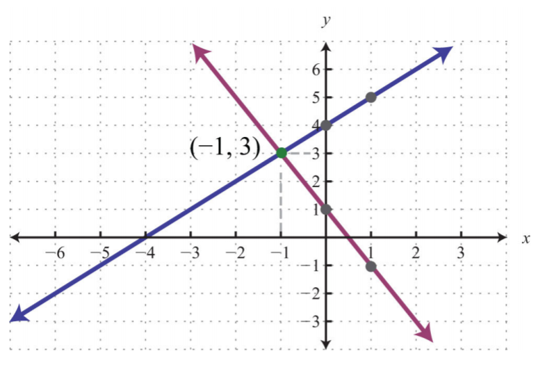
Step 2: Write the equivalent system and graph the lines on the same set of axes.
\(\begin{array}{c|c} {\color{Cerulean}{Line\:1:}\:\color{black}{y=x+4}}&{\color{Cerulean}{Line\:2}\:\color{black}{y=-2x+1}}\\{y-intercept:\:(0,4)}&{y-intercept:\:(0,1)}\\{slope:\:m=1=\frac{1}{1}=\frac{rise}{run}}&{slope:\:m=-2=\frac{-2}{1}=\frac{rise}{run}} \end{array}\)
.png?revision=1)
Step 3: Use the graph to estimate the point where the lines intersect and check to see if it solves the original system. In the above graph, the point of intersection appears to be \((−1, 3)\).
\(\color{Cerulean}{Check:}\:\color{black}{(-1,3)}\)
\(\begin{array}{c|c} {Line\:1:\:\: x-y=-4}&{Line\:2:\:\: 2x+y=1}\\{(\color{OliveGreen}{-1}\color{black}{)-(}\color{OliveGreen}{3}\color{black}{)=-4}}&{2(\color{OliveGreen}{-1}\color{black}{)+(}\color{OliveGreen}{3}\color{black}{)=1}}\\{-1-3=-4}&{-2+3=1}\\{-4=-4\quad\color{Cerulean}{\checkmark}}&{1=1\quad\color{Cerulean}{\checkmark}} \end{array}\)
Answer:
\((-1,3)\)
Solve by graphing:
\(\left\{\begin{aligned} 2x+y&=2\\−2x+3y&=−18 \end{aligned}\right.\).
Solution:
We first solve each equation for \(y\) to obtain an equivalent system where the lines are in slope-intercept form.
Graph the lines and determine the point of intersection.
\(\color{Cerulean}{Check:}\:\:\color{black}{(3,-4)}\)
\(\begin{array} {c|c} {2x+y=2}&{-2x+3y=-18}\\{2(\color{OliveGreen}{3}\color{black}{)+(}\color{OliveGreen}{-4}\color{black}{)=2}}&{-2(\color{OliveGreen}{3}\color{black}{)+3(}\color{OliveGreen}{-4}\color{black}{)=-18}}\\{6-4=2}&{-6-12=-18}\\{2=2\quad\color{Cerulean}{\checkmark}}&{-18=-18\quad\color{Cerulean}{\checkmark}} \end{array}\)
Answer:
\((3,-4)\)
Solve by graphing:
\(\left\{\begin{aligned} 3x+y&=6\\y&=−3 \end{aligned}\right.\)
Solution:
\(\color{Cerulean}{Check:}\:\color{black}{(3,-3)}\)
\(\begin{array}{c|c}{3x+y=6}&{y=-3}\\{3(\color{OliveGreen}{3}\color{black}{)+(}\color{OliveGreen}{-3}\color{black}{)=6}}&{(\color{OliveGreen}{-3}\color{black}{)=-3}}\\{9-3=6}&{-3=-3\quad\color{Cerulean}{\checkmark}}\\{6=6\quad\color{Cerulean}{\checkmark}}&{} \end{array}\)
Answer:
\((3,-3)\)
The graphing method for solving linear systems is not ideal when the solution consists of coordinates that are not integers. There will be more accurate algebraic methods in sections to come, but for now, the goal is to understand the geometry involved when solving systems. It is important to remember that the solutions to a system correspond to the point, or points, where the graphs of the equations intersect.
Solve by graphing:
\(\left\{\begin{aligned}−x+y&=6\\ 5x+2y&=−2 \end{aligned}\right.\).
- Answer
-
\((-2,4)\)
Dependent and Inconsistent Systems
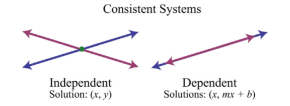
Systems with at least one solution are called consistent systems. Up to this point, all of the examples have been of consistent systems with exactly one ordered pair solution. It turns out that this is not always the case. Sometimes systems consist of two linear equations that are equivalent. If this is the case, the two lines are the same and when graphed will coincide. Hence the solution set consists of all the points on the line. This is a dependent system. Given a consistent linear system with two variables, there are two possible results:
.png?revision=1)
The solutions to independent systems are ordered pairs \((x, y)\). We need some way to express the solution sets to dependent systems, since these systems have infinitely many solutions, or points of intersection. Recall that any line can be written in slope-intercept form, \(y=mx+b\). Here, \(y\) depends on \(x\). So we may express all the ordered pair solutions \((x, y)\) in the form \((x, mx+b)\), where \(x\) is any real number.
Solve by graphing:
\(\left\{\begin{aligned}−2x+3y&=−9 \\ 4x−6y&=18\end{aligned}\right.\).
Solution:
Determine slope-intercept form for each linear equation in the system.
\(\begin{array}{c|c} {-2x+3y=-9}&{4x-6y=18}\\{-2x+3y\color{Cerulean}{+2x}\color{black}{=-9}\color{Cerulean}{+2x}}&{4x-6y\color{Cerulean}{-4x}\color{black}{=18}\color{Cerulean}{-4x}}\\{3y=2x-9}&{-6y=-4x+18}\\{\frac{3y}{\color{Cerulean}{3}}\color{black}{=\frac{2x-9}{\color{Cerulean}{3}}}}&{\frac{-6y}{\color{Cerulean}{-6}}\color{black}{=\frac{-4x+18}{\color{Cerulean}{-6}}}}\\{y=\frac{2}{3}x-3}&{y=\frac{-4}{-6}x+\frac{18}{-6}}\\{}&{y=\frac{2}{3}x-3} \end{array}\)
In slope-intercept form, we can easily see that the system consists of two lines with the same slope and same \(y\)-intercept.
They are, in fact, the same line. And the system is dependent.
Answer:
\((x,\frac{2}{3}x-3)\)
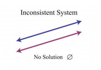
In this example, it is important to notice that the two lines have the same slope and same \(y\)-intercept. This tells us that the two equations are equivalent and that the simultaneous solutions are all the points on the line \(y=\frac{2}{3}x−3\). This is a dependent system, and the infinitely many solutions are expressed using the form \((x, mx+b)\). Other resources may express this set using set notation, \(\{(x, y) | y=\frac{2}{3}x−3\}\), which reads “the set of all ordered pairs \((x, y)\) such that \(y\) equals two-thirds \(x\) minus \(3\).” Sometimes the lines do not cross and there is no point of intersection. Such systems have no solution, \(Ø\), and are called inconsistent systems.
.png?revision=1)
Solve by graphing:
\(\left\{\begin{aligned}−2x+5y&=−15\\−4x+10y&=10\end{aligned}\right.\).
Solution:
Determine slope-intercept form for each linear equation.
\(\begin{array}{c|c} {-2x+5y=-15}&{-4x+10y=10}\\{-2x+5y\color{Cerulean}{+2x}\color{black}{=-15}\color{Cerulean}{+2x}}&{-4x+10y\color{Cerulean}{+4x}\color{black}{=10}\color{Cerulean}{+4x}}\\{5y=2x-15}&{10y=4x+10}\\{\frac{5y}{\color{Cerulean}{5}}\color{black}{=\frac{2x-15}{\color{Cerulean}{5}}}}&{\frac{10y}{\color{Cerulean}{10}}\color{black}{=\frac{4x+10}{\color{Cerulean}{10}}}}\\{y=\frac{2}{5}x-3}&{y=\frac{2}{5}x+1} \end{array}\)
In slope-intercept form, we can easily see that the system consists of two lines with the same slope and different \(y\)-intercepts.
Therefore, they are parallel and will never intersect.
Answer:
There is no simultaneous solution, \(Ø\).
Solve by graphing:
\(\left\{\begin{aligned} x+y=&−1\\−2x−2y&=2 \end{aligned}\right.\).
- Answer
-
\((x,-x-1)\)
Key Takeaways
- In this section, we limit our study to systems of two linear equations with two variables. Solutions to such systems, if they exist, consist of ordered pairs that satisfy both equations. Geometrically, solutions are the points where the graphs intersect.
- The graphing method for solving linear systems requires us to graph both of the lines on the same set of axes as a means to determine where they intersect.
- The graphing method is not the most accurate method for determining solutions, particularly when the solutions have coordinates that are not integers. It is a good practice to always check your solutions.
- Some linear systems have no simultaneous solution. These systems consist of equations that represent parallel lines with different \(y\)-intercepts and do not intersect in the plane. They are called inconsistent systems and the solution set is the empty set, \(Ø\).
- Some linear systems have infinitely many simultaneous solutions. These systems consist of equations that are equivalent and represent the same line. They are called dependent systems and their solutions are expressed using the notation \((x, mx+b)\), where \(x\) is any real number.
Determine whether the given ordered pair is a solution to the given system.
- \((3, −2); \left\{\begin{aligned} x+y&=-1\\-2x-2y&=2 \end{aligned}\right.\)
- \((−5, 0); \left\{\begin{aligned} x+y&=−1\\−2x−2y&=2 \end{aligned}\right.\)
- \((−2, −6); \left\{\begin{aligned}−x+y&=−4\\3x−y&=−12 \end{aligned}\right.\)
- \((2, −7); \left\{\begin{aligned} 3x+2y&=−8\\−5x−3y&=11 \end{aligned}\right.\)
- \((0, −3); \left\{\begin{aligned}5x−5y&=15\\−13x+2y&=−6 \end{aligned}\right.\)
- \((−12, 14); \left\{\begin{aligned} x+y&=−14\\−2x−4y&=0 \end{aligned}\right.\)
- \((\frac{3}{4}, \frac{1}{4}); \left\{\begin{aligned} −x−y&=−1\\−4x−8y&=5 \end{aligned}\right.\)
- \((−3, 4); \left\{\begin{aligned} \frac{1}{3}x+\frac{1}{2}y&=1 \\ \frac{2}{3}x−\frac{3}{2}y&=−8 \end{aligned}\right.\)
- \((−5, −3); \left\{\begin{aligned} y&=−35x−10 \\ y&=5 \end{aligned}\right.\)
- \((4, 2); \left\{\begin{aligned} x&=4−7\\x+4y&=8 \end{aligned}\right.\)
- Answer
-
1. No
3. No
5. Yes
7. No
9. Yes
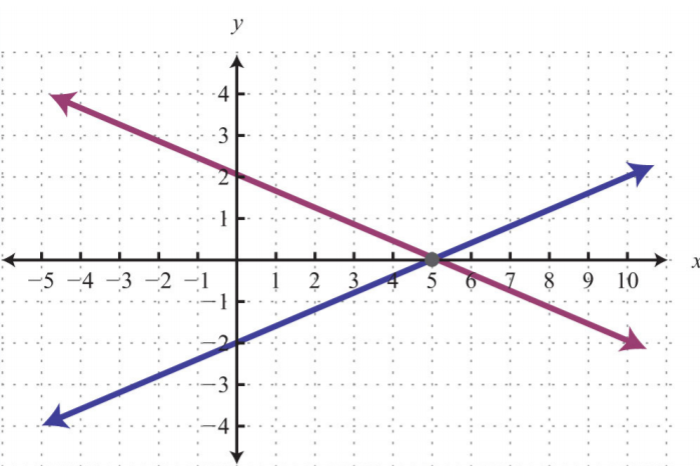
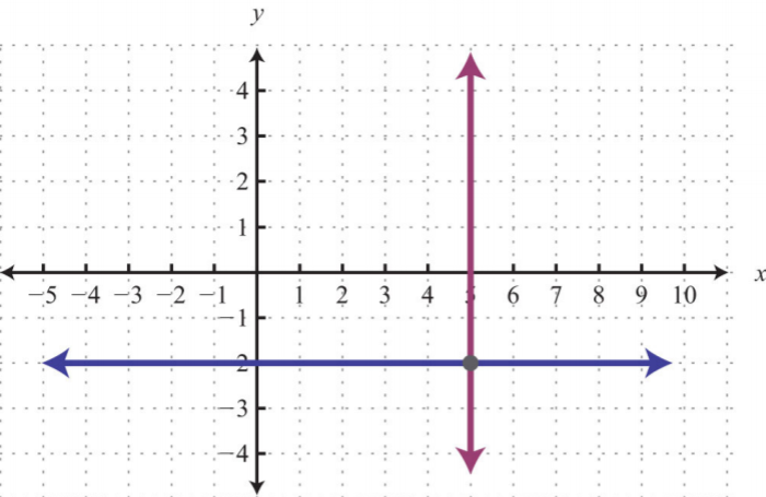
Given the graph, determine the simultaneous solution.
1.
.png?revision=1)
2.
.png?revision=1)
3.
.png?revision=1)
4.
.png?revision=1)
5.
.png?revision=1)
6.
.png?revision=1)
7.
.png?revision=1)
8.
.png?revision=1)
9.
.png?revision=1)
10.
.png?revision=1)
Figure \(\PageIndex{18}\)
- Answer
-
1. \((5, 0)\)
3. \((2, 1)\)
5. \((0, 0)\)
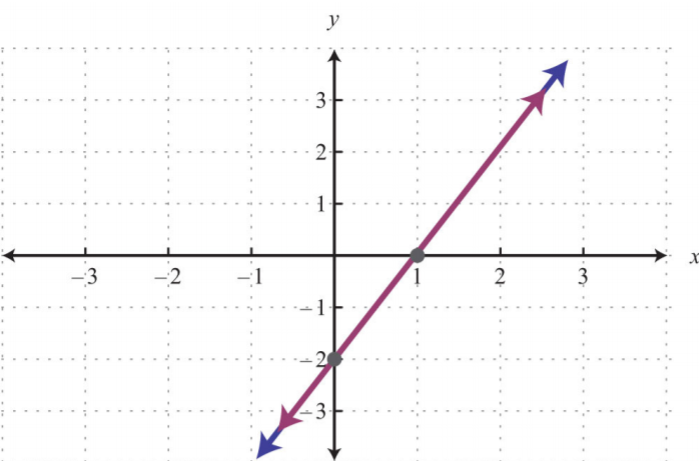
7. \((x, 2x−2)\)
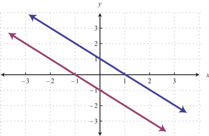
9. \(∅\)
Solve by graphing.
- \(\left\{\begin{aligned} y &=\frac{3}{2}x + 6\\y&=−x + 1 \end{aligned}\right.\)
- \(\left\{\begin{aligned} y& =\frac{3}{4}x + 2\\y&=−\frac{1}{4}x − 2 \end{aligned}\right.\)
- \(\left\{\begin{aligned} y& =x − 4\\y&=−x + 2 \end{aligned}\right.\)
- \(\left\{\begin{aligned} y&=− 5 x + 4\\y& = 4 x − 5 \end{aligned}\right.\)
- \(\left\{\begin{aligned} y& =\frac{2}{5} x + 1\\ y& =\frac{3}{5} x \end{aligned}\right.\)
- \(\left\{\begin{aligned}y&=−\frac{2}{5} x + 6\\y& =\frac{2}{5} x +10 \end{aligned}\right.\)
- \(\left\{\begin{aligned} y&=− 2\\y& =x + 1 \end{aligned}\right.\)
- \(\left\{\begin{aligned} y& = 3\\ x&=− 3 \end{aligned}\right.\)
- \(\left\{\begin{aligned} y& = 0\\y& =\frac{2}{5} x − 4 \end{aligned}\right.\)
- \(\left\{\begin{aligned} x& = 2 \\y& = 3 x \end{aligned}\right.\)
- \(\left\{\begin{aligned} y& =\frac{3}{5} x − 6\\y& =\frac{3}{5} x − 3 \end{aligned}\right.\)
- \(\left\{\begin{aligned} y&=−\frac{1}{2}x + 1\\ y&=−\frac{1}{2}x + 1 \end{aligned}\right.\)
- \(\left\{\begin{aligned}2 x + 3 y &=18 \\ − 6 x + 3 y&=− 6 \end{aligned}\right.\)
- \(\left\{\begin{aligned} − 3 x + 4y &=20\\2 x + 8y &= 8\end{aligned}\right.\)
- \(\left\{\begin{aligned} − 2 x +y &=1 \\2 x − 3 y& = 9\end{aligned}\right.\)
- \(\left\{\begin{aligned} x + 2y&=−8\\5 x + 4y&=− 4\end{aligned}\right.\)
- \(\left\{\begin{aligned}4 x + 6y &=36\\2 x − 3 y &= 6\end{aligned}\right.\)
- \(\left\{\begin{aligned} 2 x − 3 y &=18\\6 x − 3 y&=− 6\end{aligned}\right.\)
- \(\left\{\begin{aligned} 3 x + 5y &=30\\ − 6 x −10y&=−10\end{aligned}\right.\)
- \(\left\{\begin{aligned}−x + 3 y &=3\\5 x −15 y&=−15\end{aligned}\right.\)
- \(\left\{\begin{aligned}x −y &= 0\\ −x +y &= 0\end{aligned}\right.\)
- \(\left\{\begin{aligned}y &=x\\y −x& = 1\end{aligned}\right.\)
- \(\left\{\begin{aligned}3 x + 2y &= 0\\ x &= 2\end{aligned}\right.\)
- \(\left\{\begin{aligned}2 x +\frac{1}{3}y &=\frac{2}{3}\\ − 3 x +12y&=− 2\end{aligned}\right.\)
- \(\left\{\begin{aligned}\frac{1}{10}x +\frac{1}{5}y &= 2\\ −\frac{1}{5} x +\frac{1}{5}y&=− 1\end{aligned}\right.\)
- \(\left\{\begin{aligned}\frac{1}{3} x −\frac{1}{2}y &= 1 \\ \frac{1}{3} x +\frac{1}{5}y& = 1 \end{aligned}\right.\)
- \(\left\{\begin{aligned} \frac{1}{9}x +\frac{1}{6}y &= 0 \\ \frac{1}{9}x +\frac{1}{4}y &=\frac{1}{2}\end{aligned}\right.\)
- \(\left\{\begin{aligned} \frac{5}{16}x −\frac{1}{2}y &= 5\\ −\frac{5}{16}x +\frac{1}{2}y &=\frac{5}{2} \end{aligned}\right.\)
- \(\left\{\begin{aligned} \frac{1}{6}x−\frac{1}{2}y&=\frac{9}{2} \\ −\frac{1}{18}x+\frac{1}{6}y&=−\frac{3}{2} \end{aligned}\right.\)
- \(\left\{\begin{aligned} \frac{1}{2}x−\frac{1}{4}y&=−\frac{1}{2} \\ \frac{1}{3}x−\frac{1}{2}y&=3\end{aligned}\right.\)
- \(\left\{\begin{aligned} y&=4\\x&=−5 \end{aligned}\right.\)
- \(\left\{\begin{aligned} y&=−3\\x&=2\end{aligned}\right.\)
- \(\left\{\begin{aligned}y&=0\\x&=0\end{aligned}\right.\)
- \(\left\{\begin{aligned}y&=−2\\y&=3\end{aligned}\right.\)
- \(\left\{\begin{aligned}y&=5\\y&=−5\end{aligned}\right.\)
- \(\left\{\begin{aligned}y&=2\\y−2&=0\end{aligned}\right.\)
- \(\left\{\begin{aligned}x&=−5\\x&=1\end{aligned}\right.\)
- \(\left\{\begin{aligned}y&=x\\x&=0\end{aligned}\right.\)
- \(\left\{\begin{aligned}4x+6y&=3\\−x+y&=−2\end{aligned}\right.\)
- \(\left\{\begin{aligned}−2x+20y&=20\\3x+10y&=−10\end{aligned}\right.\)
- Answer
-
1. \((−2, 3)\)
3. \((3, −1)\)
5. \((5, 3)\)
7. \((−3, −2)\)
9. \((10, 0)\)
11. \(∅\)
13. \((3, 4)\)
15. \((−3, −5)\)
17. \((6, 2)\)
19. \(∅\)
21. \((x, x)\)
23. \((2, −3)\)
25. \((10, 5)\)
27. \((−9, 6)\)
29. \((x, 13x−9)\)
31. \((−5, 4)\)
33. \((0, 0)\)
35. \(∅\)
37. \(∅\)
39. \((\frac{3}{2}, −\frac{1}{2})\)
Set up a linear system of two equations and two variables and solve it using the graphing method.
- The sum of two numbers is
- The larger number is \(10\) less than five times the smaller.
- The difference between two numbers is \(12\) and their sum is \(4\).
- Where on the graph of \(3x−2y=6\) does the \(x\)-coordinate equal the \(y\)-coordinate?
- Where on the graph of \(−5x+2y=30\) does the \(x\)-coordinate equal the \(y\)-coordinate?
- Answer
-
1. The two numbers are \(5\) and \(15\).
3. \((6, 6)\)
A regional bottled water company produces and sells bottled water. The following graph depicts the supply and demand curves of bottled water in the region. The horizontal axis represents the weekly tonnage of product produced, \(Q\). The vertical axis represents the price per bottle in dollars, \(P\).
.png?revision=1)
Figure \(\PageIndex{19}\)
Use the graph to answer the following questions.
- Determine the price at which the quantity demanded is equal to the quantity supplied.
- If production of bottled water slips to \(20\) tons, then what price does the demand curve predict for a bottle of water?
- If production of bottled water increases to \(40\) tons, then what price does the demand curve predict for a bottle of water?
- If the price of bottled water is set at $\(2.50\) dollars per bottle, what quantity does the demand curve predict?
- Answer
-
1. $\(1.25\)
3. $\(1.00\)
- Discuss the weaknesses of the graphing method for solving systems.
- Explain why the solution set to a dependent linear system is denoted by \((x, mx+ b)\).
- Answer
-
1. Answers may vary