4.2: Solving Linear Systems by Substitution

Learning Objectives

• Solve linear systems using the substitution method.

The Substitution Method

In this section, we will define a completely algebraic technique for solving systems. The idea is to solve one equation for one of the variables and substitute the result into the other equation. After performing this substitution step, we will be left with a single equation with one variable, which can be solved using algebra. This is called the substitution method, and the steps are outlined in the following example.

Example \(\PageIndex{1}\)

Solve by substitution:

Solution:

Step 1: Solve for either variable in either equation. If you choose the first equation, you can isolate \(y\) in one step.

\(\begin{aligned} 2x+y&=7\\2x+y\color{Cerulean}{-2x}&=7\color{Cerulean}{-2x} \\ y&=-2x+7 \end{aligned}\)

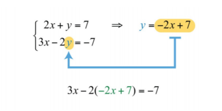
Step 2: Substitute the expression \(−2x+7\) for the \(y\) variable in the other equation.

Figure \(\PageIndex{1}\)

This leaves you with an equivalent equation with one variable, which can be solved using the techniques learned up to this point.

Step 3: Solve for the remaining variable. To solve for \(x\), first distribute \(−2\):

Step 4: Back substitute to find the value of the other coordinate. Substitute \(x= 1\) into either of the original equations or their equivalents. Typically, we use the equivalent equation that we found when isolating a variable in step 1.

\(\begin{aligned} y&=-2x+7\\&=-2(\color{OliveGreen}{1}\color{black}{)+7}\\&=-2+7\\&=5 \end{aligned}\)

The solution to the system is \((1, 5)\). Be sure to present the solution as an ordered pair.

Step 5: Check. Verify that these coordinates solve both equations of the original system:

\(\color{Cerulean}{Check:}\:\:\color{black}{(1,5)}\)

\(\begin{array}{c|c} {Equation\:1:}&{Equation\:2:}\\{2x+y=7}&{3x-2y=-7}\\{2(\color{OliveGreen}{1}\color{black}{)+(}\color{OliveGreen}{5}\color{black}{)=7}}&{3(\color{OliveGreen}{1}\color{black}{)-2(}\color{OliveGreen}{5}\color{black}{)=-7}}\\{2+5=7}&{3-10=-7}\\{7=7\quad\color{Cerulean}{\checkmark}}&{-7=-7\quad\color{Cerulean}{\checkmark}} \end{array}\)

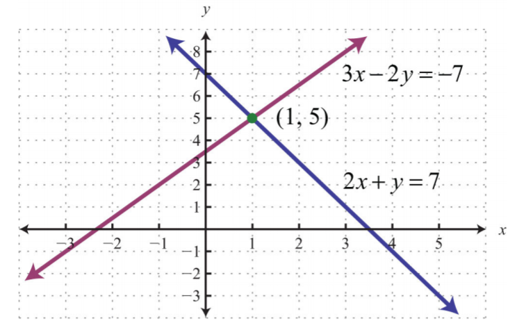
The graph of this linear system follows:

Figure \(\PageIndex{2}\)

The substitution method for solving systems is a completely algebraic method. Thus graphing the lines is not required.

Answer:

\((1, 5)\)

Example \(\PageIndex{2}\)

Solve by substitution:

\(\left\{\begin{aligned}2x−y&=1\\2x−y&=3\end{aligned}\right.\).

Solution:

In this example, we can see that \(x\) has a coefficient of \(1\) in the second equation. This indicates that it can be isolated in one step as follows:

\(\begin{aligned} x-y&=3 \\ x-y\color{Cerulean}{+y}&=3\color{Cerulean}{+y} \\ x&=3+y \end{aligned}\)

\(\left\{\begin{aligned} 2\color{Cerulean}{x}\color{black}{-y}&=12 \\ x-y&=3 \Rightarrow \color{Cerulean}{x}\color{black}{=3+y} \end{aligned} \right.\)

Substitute \(3+y\) for \(x\) in the first equation. Use parentheses and take care to distribute.

\(\begin{aligned} 2x-y&=12\\2(\color{OliveGreen}{3+y}\color{black}{)-y}&=12 \\6+2y-y&=12 \\6+y&=12 \\ 6+y\color{Cerulean}{-6}&=12\color{Cerulean}{-6}\\y&=6 \end{aligned}\)

Use \(x=3+y\) to find \(x\).

\(\begin{aligned} x&=3+y\\&=3+\color{OliveGreen}{+6}\\&=9 \end{aligned}\)

Answer:

\((9, 6)\). The check is left to the reader.

Example \(\PageIndex{3}\)

Solve by substitution:

\(\left\{\begin{aligned}3x−5y&=1\\7x&=−1\end{aligned}\right.\).

Solution:

In this example, the variable \(x\) is already isolated. Hence we can substitute \(x=−1\) into the first equation.

Answer:

\((−1, −4)\). It is a good exercise to graph this particular system to compare the substitution method to the graphing method for solving systems.

Exercise \(\PageIndex{1}\)

Solve by substitution:

\(\left\{\begin{aligned}3x+y&=4\\8x+2y&=10\end{aligned}\right.\).

Answer

\((1,1)\)

Solving systems algebraically frequently requires work with fractions.

Example \(\PageIndex{4}\)

Solve by substitution:

\(\left\{\begin{aligned}2x+8y&=5\\24x−4y&=−15\end{aligned}\right.\).

Solution:

Begin by solving for \(x\) in the first equation.

\(\begin{aligned} 2x+8y&=5\\2x+8y\color{Cerulean}{-8y}&=5\color{Cerulean}{-8y} \\ \frac{2x}{\color{Cerulean}{2}}&=\frac{-8y+5}{\color{Cerulean}{2}} \\ x&=\frac{-8y}{2}+\frac{5}{2} \\ x&=-4y+\frac{5}{2} \end{aligned}\)

\(\left\{\begin{aligned} 2x+8y&=5 \Rightarrow \color{Cerulean}{x}\color{black}{=-4y+\frac{5}{2}} \\ 24\color{Cerulean}{x}\color{black}{-4y}&=-15\end{aligned}\right.\)

Next, substitute into the second equation and solve for \(y\).

Back substitute into the equation used in the substitution step:

\(\begin{aligned} x&=-4y+\frac{5}{2} \\ &=-4\left(\color{OliveGreen}{\frac{3}{4}} \right)\color{black}{+\frac{5}{2}} \\ &=-3+\frac{5}{2} \\ &=-\frac{6}{2} + \frac{5}{2} \\ &=-\frac{1}{2} \end{aligned}\)

Answer:

\((-\frac{1}{2},\frac{3}{4})\)

As we know, not all linear systems have only one ordered pair solution. Recall that some systems have infinitely many ordered pair solutions and some do not have any solutions. Next, we explore what happens when using the substitution method to solve a dependent system.

Example \(\PageIndex{5}\)

Solve by substitution:

\(\left\{\begin{aligned}−5x+y&=−1\\10x−2y&=2\end{aligned}\right.\).

Solution:

Since the first equation has a term with coefficient \(1\), we choose to solve for that first.

Next, substitute this expression in for \(y\) in the second equation.

\(\begin{aligned} 10x-2y&=2 \\ 10x-2(\color{OliveGreen}{5x-1}\color{black}{)}&=2 \\ 10x-10x+2&=2 \\ 2&=2 \quad\color{Cerulean}{True} \end{aligned}\)

This process led to a true statement; hence the equation is an identity and any real number is a solution. This indicates that the system is dependent. The simultaneous solutions take the form \((x, mx + b)\), or in this case, \((x, 5x − 1)\), where \(x\) is any real number.

Answer:

\((x, 5x−1)\)

To have a better understanding of the previous example, rewrite both equations in slope-intercept form and graph them on the same set of axes.

Figure \(\PageIndex{3}\)

We can see that both equations represent the same line, and thus the system is dependent. Now explore what happens when solving an inconsistent system using the substitution method.

Example \(\PageIndex{6}\)

Solve by substitution:

\(\left\{\begin{aligned}−7x+3y&=3\\14x−6y&=−16\end{aligned}\right.\).

Solution:

Solve for \(y\) in the first equation.

\(\begin{aligned} -7x+3y&=3 \\ -7x+3y\color{Cerulean}{+7x}&=3\color{Cerulean}{+7x} \\3y&=7x+3 \\ \frac{3y}{\color{Cerulean}{3}}&=\frac{7x+3}{\color{Cerulean}{3}}\\y&=\frac{7}{3}x+1 \end{aligned}\)

\(\left\{\begin{aligned} -7x+3y&=3 \Rightarrow \color{Cerulean}{y}\color{black}{=\frac{7}{3}x+1} \\ 14x-6\color{Cerulean}{y}&=-16\end{aligned}\right.\)

Substitute into the second equation and solve.

Solving leads to a false statement. This indicates that the equation is a contradiction. There is no solution for \(x\) and hence no solution to the system.

Answer:

No solution, \(Ø\)

A false statement indicates that the system is inconsistent, or in geometric terms, that the lines are parallel and do not intersect. To illustrate this, determine the slope-intercept form of each line and graph them on the same set of axes.

Figure \(\PageIndex{4}\)

In slope-intercept form, it is easy to see that the two lines have the same slope but different \(y\)-intercepts.

Exercise \(\PageIndex{2}\)

Solve by substitution:

\(\left\{\begin{aligned}2x−5y&=3\\4x−10y&=6\end{aligned}\right.\).

Answer

\((x, \frac{2}{5}x−\frac{3}{5}) \)

Key Takeaways

• The substitution method is a completely algebraic method for solving a system of equations.
• The substitution method requires that we solve for one of the variables and then substitute the result into the other equation. After performing the substitution step, the resulting equation has one variable and can be solved using the techniques learned up to this point.
• When the value of one of the variables is determined, go back and substitute it into one of the original equations, or their equivalent equations, to determine the corresponding value of the other variable.
• Solutions to systems of two linear equations with two variables, if they exist, are ordered pairs \((x, y)\).
• If the process of solving a system of equations leads to a false statement, then the system is inconsistent and there is no solution, \(Ø\).
• If the process of solving a system of equations leads to a true statement, then the system is dependent and there are infinitely many solutions that can be expressed using the form \((x, mx + b)\).

Exercise \(\PageIndex{3}\) Substitution Method

Solve by substitution.

1. \(\left\{\begin{aligned} y&=4x−1\\−3x+y&=1\end{aligned}\right.\)
2. \(\left\{\begin{aligned}y&=3x−8\\4x−y&=2 \end{aligned}\right.\)
3. \(\left\{\begin{aligned}x&=2y−3\\x+3y&=−8 \end{aligned}\right.\)
4. \(\left\{\begin{aligned}x&=−4y+12\\x+3y&=12 \end{aligned}\right.\)
5. \(\left\{\begin{aligned}y&=3x−5\\x+2y&=2 \end{aligned}\right.\)
6. \(\left\{\begin{aligned}y&=x\\2x+3y&=10 \end{aligned}\right.\)
7. \(\left\{\begin{aligned}y&=4x+1\\−4x+y&=2 \end{aligned}\right.\)
8. \(\left\{\begin{aligned}y&=−3x+5\\3x+y&=5 \end{aligned}\right.\)
9. \(\left\{\begin{aligned}y&=2x+3\\2x−y&=−3 \end{aligned}\right.\)
10. \(\left\{\begin{aligned}y&=5x−1\\x−2y&=5 \end{aligned}\right.\)
11. \(\left\{\begin{aligned}y&=−7x+1\\3x−y&=4 \end{aligned}\right.\)
12. \(\left\{\begin{aligned}x&=6y+2\\5x−2y&=0 \end{aligned}\right.\)
13. \(\left\{\begin{aligned}y&=−2−2x\\−y&=−6 \end{aligned}\right.\)
14. \(\left\{\begin{aligned}x&=−3x−4\\y&=−3 \end{aligned}\right.\)
15. \(\left\{\begin{aligned}y&=−\frac{1}{5}x+\frac{3}{7}\\x−5y&=9 \end{aligned}\right.\)
16. \(\left\{\begin{aligned}y&=\frac{2}{3}x−\frac{1}{6}\\x−9y&=0 \end{aligned}\right.\)
17. \(\left\{\begin{aligned}y&=\frac{1}{2}x+\frac{1}{3}\\x−6y&=4 \end{aligned}\right.\)
18. \(\left\{\begin{aligned}y&=−\frac{3}{8}x+\frac{1}{2}\\2x+4y&=1 \end{aligned}\right.\)
19. \(\left\{\begin{aligned}x+y&=6\\2x+3y=\frac{1}{6} \end{aligned}\right.\)
20. \(\left\{\begin{aligned}x−y&=3\\−2x+3y&=−2 \end{aligned}\right.\)
21. \(\left\{\begin{aligned}2x+y&=2\\3x−2y&=\frac{1}{7} \end{aligned}\right.\)
22. \(\left\{\begin{aligned}x−3y&=−\frac{1}{13}\\x+5y&=−5 \end{aligned}\right.\)
23. \(\left\{\begin{aligned}x+2y&=−3\\3x−4y&=−2 \end{aligned}\right.\)
24. \(\left\{\begin{aligned}5x−y&=12\\9x−y&=10 \end{aligned}\right.\)
25. \(\left\{\begin{aligned}x+2y&=−6\\−4x−8y&=24 \end{aligned}\right.\)
26. \(\left\{\begin{aligned}x+3y&=−6\\−2x−6y&=−12 \end{aligned}\right.\)
27. \(\left\{\begin{aligned}−3x+y&=−4\\6x−2y&=−2 \end{aligned}\right.\)
28. \(\left\{\begin{aligned}x−5y&=−10\\2x−10y&=−20 \end{aligned}\right.\)
29. \(\left\{\begin{aligned}3x−y&=9\\4x+3y&=−1 \end{aligned}\right.\)
30. \(\left\{\begin{aligned}2x−y&=5\\4x+2y&=−2 \end{aligned}\right.\)
31. \(\left\{\begin{aligned}−x+4y&=0\\2x−5y&=−6 \end{aligned}\right.\)
32. \(\left\{\begin{aligned}3y−x&=5\\5x+2y&=−8 \end{aligned}\right.\)
33. \(\left\{\begin{aligned}2x−5y&=1\\4x+10y&=2 \end{aligned}\right.\)
34. \(\left\{\begin{aligned}3x−7y&=−3\\6x+14y&=0 \end{aligned}\right.\)
35. \(\left\{\begin{aligned}10x−y&=3\\−5x+12y&=1 \end{aligned}\right.\)
36. \(\left\{\begin{aligned}−\frac{1}{3}x+\frac{1}{6}y&=\frac{2}{3}\\ \frac{1}{2}x−\frac{1}{3}y&=−\frac{3}{2} \end{aligned}\right.\)
37. \(\left\{\begin{aligned}\frac{1}{3}x+\frac{2}{3}y&=1 \\ \frac{1}{4}x−\frac{1}{3}y&=−\frac{1}{12} \end{aligned}\right.\)
38. \(\left\{\begin{aligned}\frac{1}{7}x−y&=\frac{1}{2}\\ \frac{1}{4}x+\frac{1}{2}y&=2 \end{aligned}\right.\)
39. \(\left\{\begin{aligned}−\frac{3}{5}x+\frac{2}{5}y&=\frac{1}{2}\\ \frac{1}{3}x−\frac{1}{12}y&=−\frac{1}{3} \end{aligned}\right.\)
40. \(\left\{\begin{aligned}\frac{1}{2}x&=\frac{2}{3}y\\x−\frac{2}{3}y&=2 \end{aligned}\right.\)
41. \(\left\{\begin{aligned}−\frac{1}{2}x+\frac{1}{2}y&=\frac{5}{8} \\ \frac{1}{4}x+\frac{1}{2}y&=\frac{1}{4} \end{aligned}\right.\)
42. \(\left\{\begin{aligned}x−y&=0\\−x+2y&=3 \end{aligned}\right.\)
43. \(\left\{\begin{aligned}y&=3x\\2x−3y&=0 \end{aligned}\right.\)
44. \(\left\{\begin{aligned}2x+3y&=18\\−6x+3y&=−6 \end{aligned}\right.\)
45. \(\left\{\begin{aligned}−3x+4y&=20\\ 2x+8y&=8 \end{aligned}\right.\)
46. \(\left\{\begin{aligned}5x−3y&=−1\\ 3x+2y&=7 \end{aligned}\right.\)
47. \(\left\{\begin{aligned}−3x+7y&=2\\ 2x+7y&=1 \end{aligned}\right.\)
48. \(\left\{\begin{aligned}y&=3\\y&=−3 \end{aligned}\right.\)
49. \(\left\{\begin{aligned}x&=5\\x&=−2 \end{aligned}\right.\)
50. \(\left\{\begin{aligned}y&=4\\y&=4\end{aligned}\right.\)

Answer

1. \((2, 7)\)

3. \((−5, −1)\)

5. \((2, 6)\)

7. \(∅\)

9. \((x, 2x+3)\)

11. \((\frac{1}{2}, −\frac{5}{2})\)

13. \((4, −2)\)

15. \((3, \frac{12}{5})\)

17. \((−3, −\frac{7}{6})\)

19. \((2, 4)\)

21. \((3, −4)\)

23. \((−\frac{8}{5}, −\frac{7}{10})\)

25. \((x, −\frac{1}{2}x−3)\)

27. \(∅\)

29. \((2, −3)\)

31. \((−8, −2)\)

33. \((\frac{1}{2}, 0)\)

35. \(∅\)

37. \((1, 1)\)

39. \((−\frac{11}{10}, −\frac{2}{5})\)

41. \((−\frac{1}{2}, \frac{3}{4})\)

43. \((0, 0)\)

45. \((−4, 2)\)

47. \((−\frac{1}{5}, \frac{1}{5})\)

49. \(∅\)

Exercise \(\PageIndex{4}\) Substitution Method

Set up a linear system and solve it using the substitution method.

1. The sum of two numbers is \(19\). The larger number is \(1\) less than three times the smaller.
2. The sum of two numbers is \(15\). The larger is \(3\) more than twice the smaller.
3. The difference of two numbers is \(7\) and their sum is \(1\).
4. The difference of two numbers is \(3\) and their sum is \(−7\).
5. Where on the graph of \(−5x+3y=30\) does the \(x\)-coordinate equal the \(y\)-coordinate?
6. Where on the graph of \(\frac{1}{2}x−\frac{1}{3}y=1\) does the \(x\)-coordinate equal the \(y\)-coordinate?

Answer

1. The two numbers are \(5\) and \(14\).

3. The two numbers are \(4\) and \(−3\).

5. \((−\frac{1}{5}, −\frac{1}{5})\)

Exercise \(\PageIndex{5}\) Discussion Board Topics

1. Describe what drives the choice of variable to solve for when beginning the process of solving by substitution.
2. Discuss the merits and drawbacks of the substitution method.

Answer

1. Answers may vary