
4.1: Piecewise-Defined Functions
- Page ID
- 19699

\( \newcommand{\vecs}[1]{\overset { \scriptstyle \rightharpoonup} {\mathbf{#1}} } \)
\( \newcommand{\vecd}[1]{\overset{-\!-\!\rightharpoonup}{\vphantom{a}\smash {#1}}} \)
\( \newcommand{\dsum}{\displaystyle\sum\limits} \)
\( \newcommand{\dint}{\displaystyle\int\limits} \)
\( \newcommand{\dlim}{\displaystyle\lim\limits} \)
\( \newcommand{\id}{\mathrm{id}}\) \( \newcommand{\Span}{\mathrm{span}}\)
( \newcommand{\kernel}{\mathrm{null}\,}\) \( \newcommand{\range}{\mathrm{range}\,}\)
\( \newcommand{\RealPart}{\mathrm{Re}}\) \( \newcommand{\ImaginaryPart}{\mathrm{Im}}\)
\( \newcommand{\Argument}{\mathrm{Arg}}\) \( \newcommand{\norm}[1]{\| #1 \|}\)
\( \newcommand{\inner}[2]{\langle #1, #2 \rangle}\)
\( \newcommand{\Span}{\mathrm{span}}\)
\( \newcommand{\id}{\mathrm{id}}\)
\( \newcommand{\Span}{\mathrm{span}}\)
\( \newcommand{\kernel}{\mathrm{null}\,}\)
\( \newcommand{\range}{\mathrm{range}\,}\)
\( \newcommand{\RealPart}{\mathrm{Re}}\)
\( \newcommand{\ImaginaryPart}{\mathrm{Im}}\)
\( \newcommand{\Argument}{\mathrm{Arg}}\)
\( \newcommand{\norm}[1]{\| #1 \|}\)
\( \newcommand{\inner}[2]{\langle #1, #2 \rangle}\)
\( \newcommand{\Span}{\mathrm{span}}\) \( \newcommand{\AA}{\unicode[.8,0]{x212B}}\)
\( \newcommand{\vectorA}[1]{\vec{#1}} % arrow\)
\( \newcommand{\vectorAt}[1]{\vec{\text{#1}}} % arrow\)
\( \newcommand{\vectorB}[1]{\overset { \scriptstyle \rightharpoonup} {\mathbf{#1}} } \)
\( \newcommand{\vectorC}[1]{\textbf{#1}} \)
\( \newcommand{\vectorD}[1]{\overrightarrow{#1}} \)
\( \newcommand{\vectorDt}[1]{\overrightarrow{\text{#1}}} \)
\( \newcommand{\vectE}[1]{\overset{-\!-\!\rightharpoonup}{\vphantom{a}\smash{\mathbf {#1}}}} \)
\( \newcommand{\vecs}[1]{\overset { \scriptstyle \rightharpoonup} {\mathbf{#1}} } \)
\(\newcommand{\longvect}{\overrightarrow}\)
\( \newcommand{\vecd}[1]{\overset{-\!-\!\rightharpoonup}{\vphantom{a}\smash {#1}}} \)
\(\newcommand{\avec}{\mathbf a}\) \(\newcommand{\bvec}{\mathbf b}\) \(\newcommand{\cvec}{\mathbf c}\) \(\newcommand{\dvec}{\mathbf d}\) \(\newcommand{\dtil}{\widetilde{\mathbf d}}\) \(\newcommand{\evec}{\mathbf e}\) \(\newcommand{\fvec}{\mathbf f}\) \(\newcommand{\nvec}{\mathbf n}\) \(\newcommand{\pvec}{\mathbf p}\) \(\newcommand{\qvec}{\mathbf q}\) \(\newcommand{\svec}{\mathbf s}\) \(\newcommand{\tvec}{\mathbf t}\) \(\newcommand{\uvec}{\mathbf u}\) \(\newcommand{\vvec}{\mathbf v}\) \(\newcommand{\wvec}{\mathbf w}\) \(\newcommand{\xvec}{\mathbf x}\) \(\newcommand{\yvec}{\mathbf y}\) \(\newcommand{\zvec}{\mathbf z}\) \(\newcommand{\rvec}{\mathbf r}\) \(\newcommand{\mvec}{\mathbf m}\) \(\newcommand{\zerovec}{\mathbf 0}\) \(\newcommand{\onevec}{\mathbf 1}\) \(\newcommand{\real}{\mathbb R}\) \(\newcommand{\twovec}[2]{\left[\begin{array}{r}#1 \\ #2 \end{array}\right]}\) \(\newcommand{\ctwovec}[2]{\left[\begin{array}{c}#1 \\ #2 \end{array}\right]}\) \(\newcommand{\threevec}[3]{\left[\begin{array}{r}#1 \\ #2 \\ #3 \end{array}\right]}\) \(\newcommand{\cthreevec}[3]{\left[\begin{array}{c}#1 \\ #2 \\ #3 \end{array}\right]}\) \(\newcommand{\fourvec}[4]{\left[\begin{array}{r}#1 \\ #2 \\ #3 \\ #4 \end{array}\right]}\) \(\newcommand{\cfourvec}[4]{\left[\begin{array}{c}#1 \\ #2 \\ #3 \\ #4 \end{array}\right]}\) \(\newcommand{\fivevec}[5]{\left[\begin{array}{r}#1 \\ #2 \\ #3 \\ #4 \\ #5 \\ \end{array}\right]}\) \(\newcommand{\cfivevec}[5]{\left[\begin{array}{c}#1 \\ #2 \\ #3 \\ #4 \\ #5 \\ \end{array}\right]}\) \(\newcommand{\mattwo}[4]{\left[\begin{array}{rr}#1 \amp #2 \\ #3 \amp #4 \\ \end{array}\right]}\) \(\newcommand{\laspan}[1]{\text{Span}\{#1\}}\) \(\newcommand{\bcal}{\cal B}\) \(\newcommand{\ccal}{\cal C}\) \(\newcommand{\scal}{\cal S}\) \(\newcommand{\wcal}{\cal W}\) \(\newcommand{\ecal}{\cal E}\) \(\newcommand{\coords}[2]{\left\{#1\right\}_{#2}}\) \(\newcommand{\gray}[1]{\color{gray}{#1}}\) \(\newcommand{\lgray}[1]{\color{lightgray}{#1}}\) \(\newcommand{\rank}{\operatorname{rank}}\) \(\newcommand{\row}{\text{Row}}\) \(\newcommand{\col}{\text{Col}}\) \(\renewcommand{\row}{\text{Row}}\) \(\newcommand{\nul}{\text{Nul}}\) \(\newcommand{\var}{\text{Var}}\) \(\newcommand{\corr}{\text{corr}}\) \(\newcommand{\len}[1]{\left|#1\right|}\) \(\newcommand{\bbar}{\overline{\bvec}}\) \(\newcommand{\bhat}{\widehat{\bvec}}\) \(\newcommand{\bperp}{\bvec^\perp}\) \(\newcommand{\xhat}{\widehat{\xvec}}\) \(\newcommand{\vhat}{\widehat{\vvec}}\) \(\newcommand{\uhat}{\widehat{\uvec}}\) \(\newcommand{\what}{\widehat{\wvec}}\) \(\newcommand{\Sighat}{\widehat{\Sigma}}\) \(\newcommand{\lt}{<}\) \(\newcommand{\gt}{>}\) \(\newcommand{\amp}{&}\) \(\definecolor{fillinmathshade}{gray}{0.9}\)In preparation for the definition of the absolute value function, it is extremely important to have a good grasp of the concept of a piecewise-defined function. However, before we jump into the fray, let’s take a look at a special type of function called a constant function.
One way of understanding a constant function is to have a look at its graph.
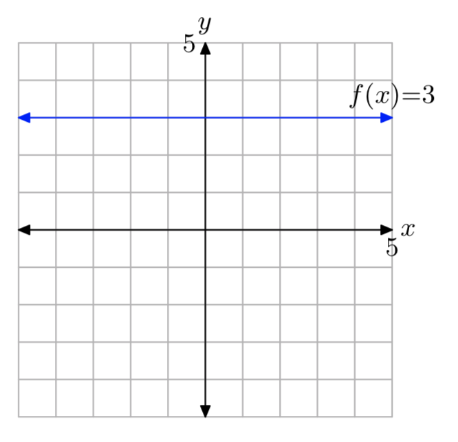
Sketch the graph of the constant function f(x) = 3.
Solution
Because the notation f(x) = 3 is equivalent to the notation y = 3, we can sketch a graph of f by drawing the graph of the horizontal line having equation y = 3, as shown in Figure \(\PageIndex{1}\).
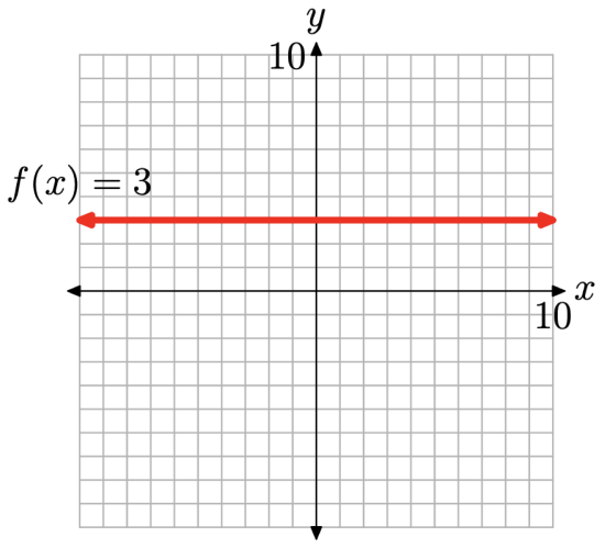
When you look at the graph in Figure 1, note that every point on the horizontal line having equation f(x) = 3 has a y-value equal to 3. We say that the y-values on this horizontal line are constant, for the simple reason that they are constantly equal to 3.
The function form works in precisely the same manner. Look again at the notation \[f(x)=3 \nonumber \]
Note that no matter what number you substitute for x in the left-hand side of f(x) = 3, the right-hand side is constantly equal to 3. Thus,
\[f(-5)=3, \quad f(-1 / 2)=3, \quad f(\sqrt{2})=3, \quad \text { or } \quad f(\pi)=3 \nonumber \]
The above discussion leads to the following definition.
The function defined by f(x) = c, where c is a constant (fixed real number), is called a constant function.
Two comments are in order:
- f(x) = c for all real numbers x.
- The graph of f(x) = c is a horizontal line. It consists of all the points (x, y) having y-value equal to c.
Piecewise Constant Functions
Piecewise functions are a favorite of engineers. Let’s look at an example.
Suppose that a battery provides no voltage to a circuit when a switch is open. Then, starting at time \(t = 0\), the switch is closed and the battery provides a constant 5 volts from that time forward. Create a piecewise function modeling the problem constraints and sketch its graph.
Solution
This is a fairly simple exercise, but we will have to introduce some new notation. First of all, if the time t is less than zero (\(t < 0\)), then the voltage is 0 volts. If the time t is greater than or equal to zero (\(t \geq 0\)), then the voltage is a constant 5 volts. Here is the notation we will use to summarize this description of the voltage.
\[V(t)=\left\{\begin{array}{ll}{0,} & {\text { if } t<0} \\ {5,} & {\text { if } t \geq 0}\end{array}\right. \nonumber \]
Some comments are in order:
- The voltage difference provide by the battery in the circuit is a function of time. Thus, V (t) represents the voltage at time t.
- The notation used in (4) is universally adopted by mathematicians in situations where the function changes definition depending on the value of the independent variable. This definition of the function V is called a “piecewise definition.” Because each of the pieces in this definition is constant, the function V is called a piecewise constant function.
- This particular function has two pieces. The function is the constant function \(V (t) = 0\), when \(t < 0\), but a different constant function, \(V (t) = 5\), when \(t \geq 0\).
If \(t<0, V(t)=0 .\) For example, for \(t=-1, t=-10,\) and \(t=-100\)
\[V(-1)=0, \quad V(-10)=0, \quad \text { and } \quad V(-100)=0 \nonumber \]
On the other hand, if \(t \geq 0,\) then \(V(t)=5 .\) For example, for \(t=0, t=10,\) and \(t=100\)
\[V(0)=5, \quad V(10)=5, \quad \text { and } \quad V(100)=5 \nonumber \]
Before we present the graph of the piecewise constant function V , let’s pause for a moment to make sure we understand some standard geometrical terms.
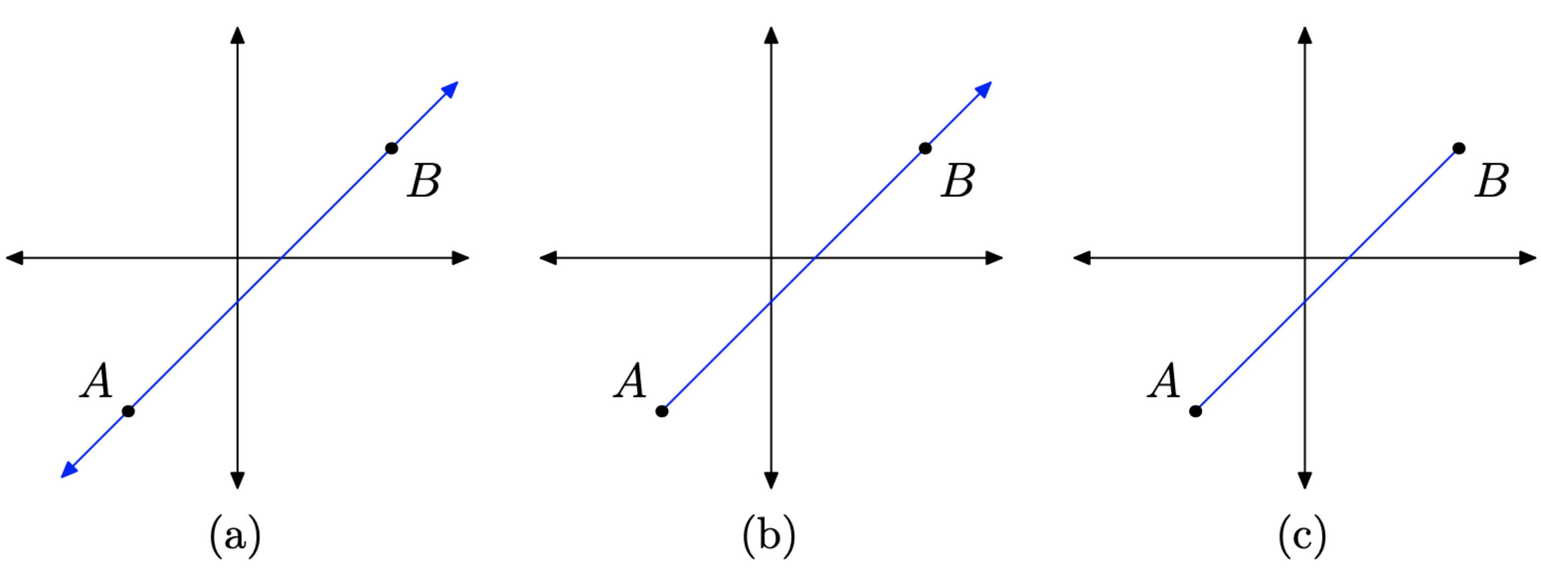
- A line stretches indefinitely in two directions, as shown in Figure \(\PageIndex{2}\)(a).
- If a line has a fixed endpoint and stretches indefinitely in only one direction, as shown in Figure \(\PageIndex{2}\)(b), then it is called a ray.
- If a portion of the line is fixed at each end, as shown in Figure \(\PageIndex{2}\)(c), then it is called a line segment.
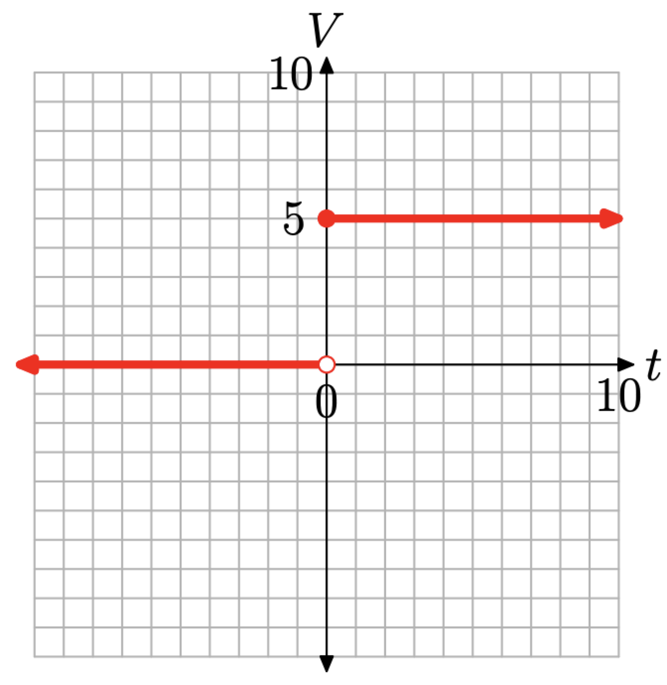
With these terms in hand, let’s turn our attention to the graph of the voltage defined by equation (4). When \(t < 0\), then \(V (t) = 0\). Normally, the graph of \(V (t) = 0\) would be a horizontal line where each point on the line has V -value equal to zero. However, \(V (t) = 0\) only if \(t < 0\), so the graph is the horizontal ray that starts at the origin, then moves indefinitely to the left, as shown in Figure \(\PageIndex{3}\). That is, the horizontal line \(V = 0\) has been restricted to the domain \(\{t : t<0\}\) and exists only to the left of the origin.
Similarly, when \(t \geq 0\), then \(V (t) = 5\) is the horizontal ray shown in Figure \(\PageIndex{3}\). Each point on the ray has a V -value equal to 5.
Two comments are in order:
- Because \(V (t) = 0\) only when t < 0, the point (0, 0) is unfilled (it is an open circle). The open circle at (0, 0) is a mathematician’s way of saying that this particular point is not plotted or shaded.
- Because \(V (t) = 5\) when \(t \geq 0\), the point (0, 5) is filled (it is a filled circle). The filled circle at (0, 5) is a mathematician’s way of saying that this particular point is plotted or shaded.
Let’s look at another example.
Consider the piecewise-defined function
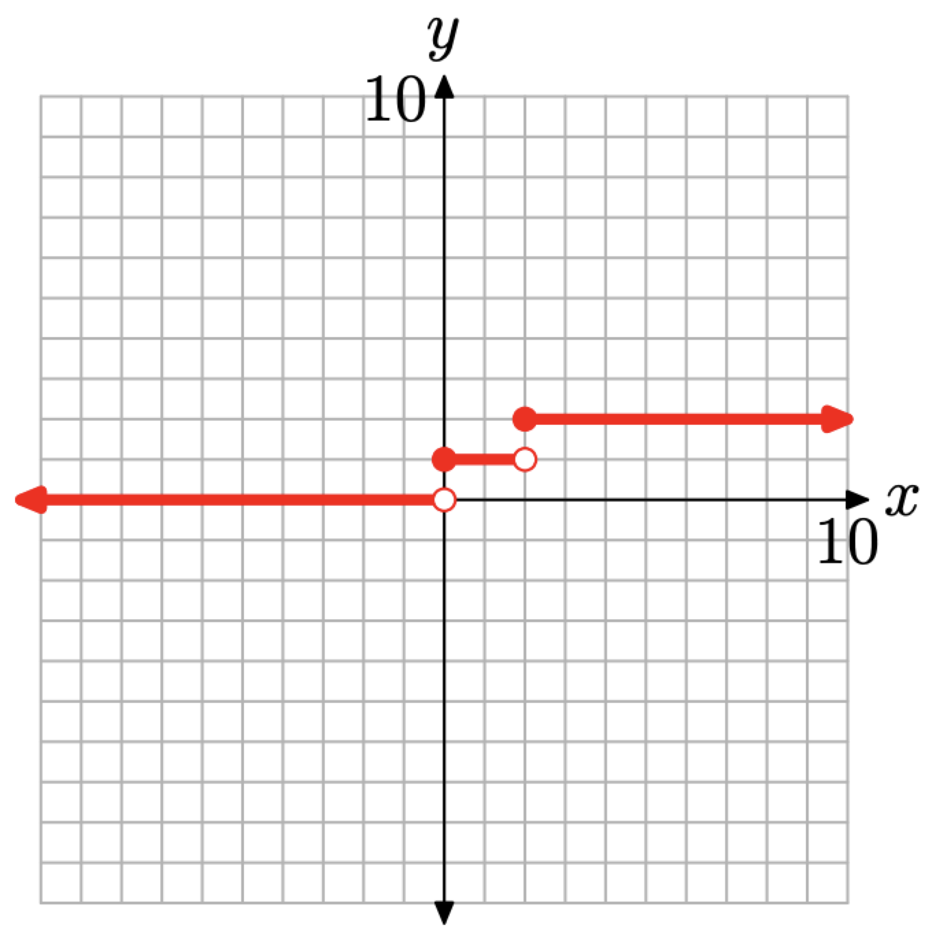
\[f(x)=\left\{\begin{array}{ll}{0,} & {\text { if } x<0} \\ {1,} & {\text { if } 0 \leq x<2} \\ {2,} & {\text { if } x \geq 2}\end{array}\right. \nonumber \]
Evaluate f(x) at x = −1, 0, 1, 2, and 3. Sketch the graph of the piecewise function f.
Solution
Because each piece of the function in (6) is constant, evaluation of the function is pretty easy. You just have to select the correct piece.
• Note that x = −1 is less than 0, so we use the first piece and write f(−1) = 0.
• Note that x = 0 satisfies \(0 \leq x<2\), so we use the second piece and write f(0) = 1.
• Note that x = 1 satisfies \(0 \leq x<2\), so we use the second piece and write f(1) = 1.
• Note that x = 2 satisfies \(x \geq 2\), so we use the third piece and write f(2) = 2.
• Finally, note that x = 3 satisfies \(x \geq 2\), so we use the third piece and write f(3) = 2. The graph is just as simple to sketch.
• Because f(x) = 0 for x < 0, the graph of this piece is a horizontal ray with endpoint at x = 0. Each point on this ray will have a y-value equal to zero and the ray will lie entirely to the left of x = 0, as shown in Figure \(\PageIndex{4}\).
• Because f(x) = 1 for \(0 \leq x<2\), the graph of this piece is a horizontal segment with one endpoint at x = 0 and the other at x = 2. Each point on this segment will have a y-value equal to 1, as shown in Figure \(\PageIndex{4}\).
• Because f(x) = 2 for \(x \geq 2\), the graph of this piece is a horizontal ray with endpoint at x = 2. Each point on this ray has a y-value equal to 2 and the ray lies entirely to the right of x = 2, as shown in Figure \(\PageIndex{4}\).
Several remarks are in order:
• The function is zero to the left of the origin (for x < 0), but not at the origin. This is indicated by an empty circle at the origin, an indication that we are not plotting that particular point.
• For \(0 \leq x<2\), the function equals 1. That is, the function is constantly equal to 1 for all values of x between 0 and 2, including zero but not including 2. This is why you see a filled circle at (0, 1) and an empty circle at (2, 1).
• Finally, for \(x \geq 2\), the function equals 2. That is, the function is constantly equal to 2 whenever x is greater than or equal to 2. That is why you see a filled circle at (2, 2).
Piecewise-Defined Functions
Now, let’s look at a more generic situation involving piecewise-defined functions—one where the pieces are not necessarily constant. The best way to learn is by doing, so let’s start with an example.
Consider the piecewise-defined function
\[f(x)=\left\{\begin{array}{ll}{-x+2,} & {\text { if } x<2} \\ {x-2,} & {\text { if } x \geq 2}\end{array}\right. \nonumber \]
Evaluate f(x) for x = 0, 1, 2, 3 and 4, then sketch the graph of the piecewise-defined function.
Solution
The function changes definition at x = 2. If x < 2, then f(x) = −x + 2. Because both 0 and 1 are strictly less than 2, we evaluate the function with this first piece of the definition.
\[\begin{array}{ll}{f(x)=-x+2} &\text{and} & {f(x)=-x+2} \\ {f(0)=-0+2} & &{f(1)=-1+2} \\ {f(0)=2} & &{f(1)=1}\end{array} \nonumber \]
On the other hand, if \(x \geq 2\), then \(f(x) = x − 2\). Because 2, 3, and 4 are all greater than or equal to 2, we evaluate the function with this second piece of the definition.
\[\begin{array}{lll}{f(x)=x-2}&{\text { and }} & {f(x)=x-2} & {\text { and }} & {f(x)=x-2} \\ {f(2)=2-2} &{\text { and }}& {f(3)=3-2} &{\text { and }}& {f(4)=4-2} \\ {f(2)=0} &{\text { and }}& {f(3)=1} & {\text { and }}&{f(4)=2}\end{array} \nonumber \]
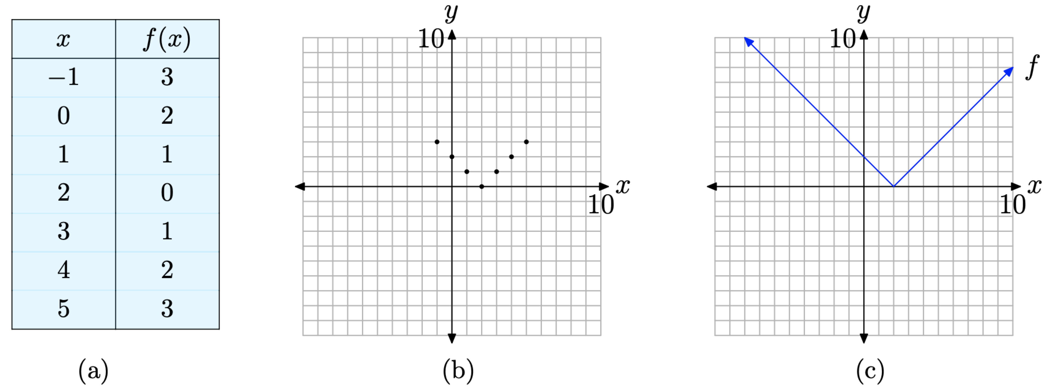
One possible approach to the graph of f is to place the points we’ve already calculated, plus a couple extra, in a table (see Figure \(\PageIndex{5}\)(a)), plot them (see Figure \(\PageIndex{5}\)(b)), then intuit the shape of the graph from the evidence provided by the plotted points. This is done in Figure \(\PageIndex{5}\)(c).
However pragmatic, this point-plotting approach is a bit tedious; but, more importantly, it does not provide the background necessary for the discussion of the absolute value function in the next section. We need to stretch our understanding to a higher level. Fortunately, all the groundwork is in place. We need only apply what we already know about the equations of lines to fit this piecewise situation.
Alternative approach. Let’s use our knowledge of the equation of a line (i.e. y = mx + b) to help sketch the graph of the piecewise function defined in (8).
Let’s sketch the first piece of the function f defined in (8). We have f(x) = −x+ 2, provided x < 2. Normally, this would be a line (with slope −1 and intercept 2), but we are to sketch only a part of that line, the part where x < 2 (x is to the left of 2). Thus, this piece of the graph will be a ray, starting at the point where x = 2, then moving indefinitely to the left.
The easiest way to sketch a ray is to first calculate and plot its fixed endpoint (in this case at x = 2), then plot a second point on the ray having x-value less than 2, then use a ruler to draw the ray.
With this thought in mind, to find the coordinates of the endpoint of the ray, substitute x = 2 in f(x) = −x + 2 to get f(2) = 0. Now, technically, we’re not supposed to use this piece of the function unless x is strictly less than 2, but we could use it with x = 1.9, or x = 1.99, or x = 1.999, etc. So let’s go ahead and use x = 2 in this piece of the function, but indicate that we’re not actually supposed to use this point by drawing an “empty circle” at (2, 0), as shown in Figure \(\PageIndex{6}\)(a).
To complete the plot of the ray, we need a second point that lies to the left of its endpoint at (2, 0). Note that x = 0 is to the left of x = 2. Evaluate f(x) = −x + 2 at x = 0 to obtain f(0) = −0 + 2 = 2. This gives us the second point (0, 2), which we plot as shown in Figure \(\PageIndex{6}\)(a). Finally, draw the ray with endpoint at (2, 0) and second point at (0, 2), as shown in Figure \(\PageIndex{6}\)(a).
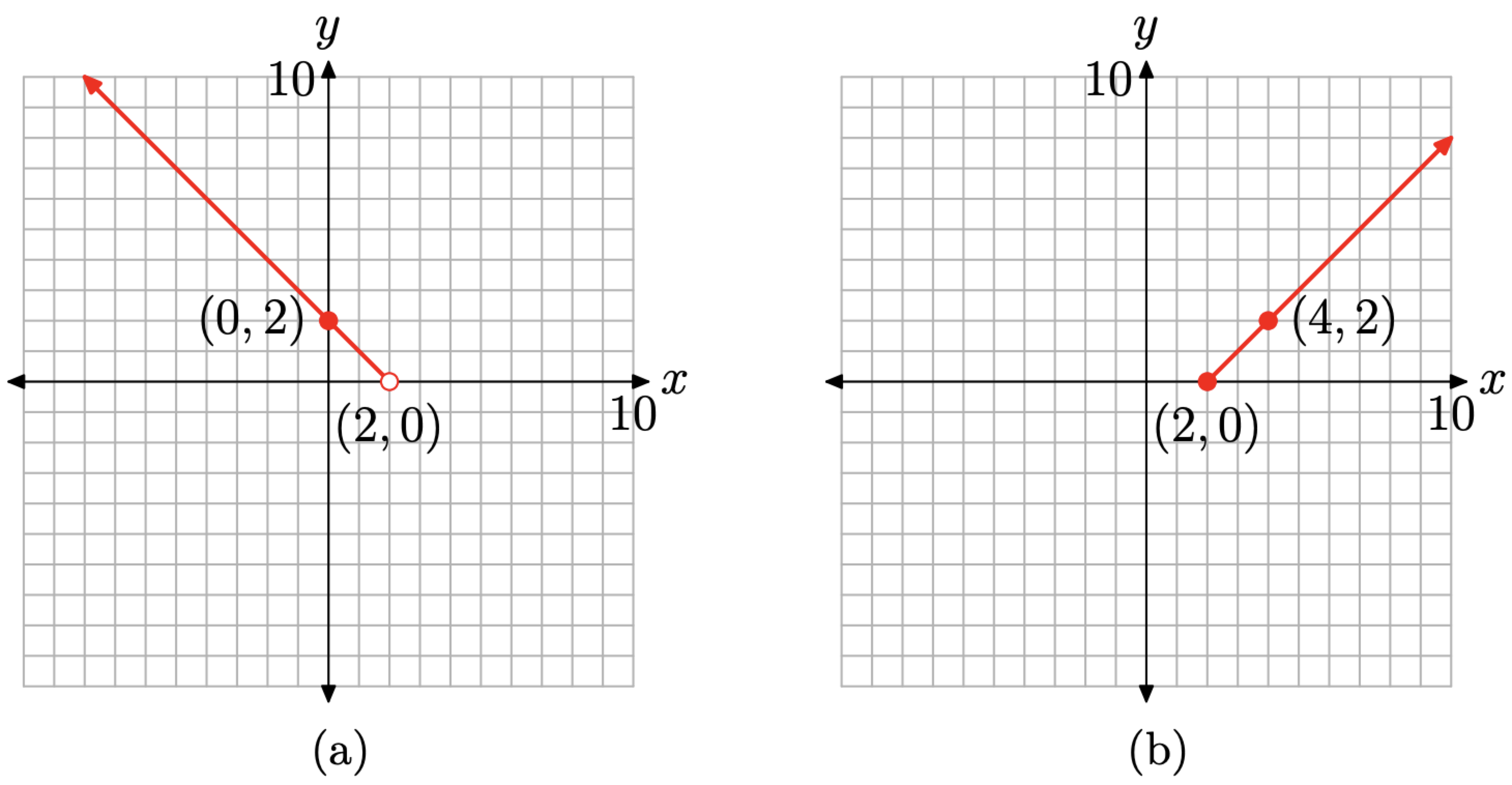
We now repeat this process for the second piece of the function defined in (8). The equation of the second piece is f(x) = x − 2, provided \(x \geq 2\). Normally, f(x) = x − 2 would be a line (with slope 1 and intercept −2), but we’re only supposed to sketch that part of the line that lies to the right of or at x = 2. Thus, the graph of this second piece is a ray, starting at the point with x = 2 and continuing to the right. If we evaluate f(x) = x − 2 at x = 2, then f(2) = 2 − 2 = 0. Thus, the fixed endpoint of the ray is at the point (2, 0). Since we’re actually supposed to use this piece with x = 2, we indicate this fact with a filled circle at (2, 0), as shown in Figure \(\PageIndex{6}\)(b).
We need a second point to the right of this fixed endpoint, so we evaluate f(x) = x−2 at x = 4 to get f(4) = 4 − 2 = 2. Thus, a second point on the ray is the point (4, 2). Finally, we simply draw the ray, starting at the endpoint (2, 0) and passing through the second point at (4, 2), as shown in Figure \(\PageIndex{6}\)(b).
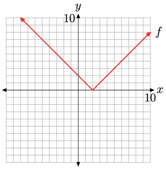
To complete the graph of the piecewise function f defined in equation (8), simply combine the two pieces in Figure \(\PageIndex{6}\)(a) and Figure \(\PageIndex{6}\)(b) to get the finished graph in Figure \(\PageIndex{7}\). Note that the graph in Figure \(\PageIndex{7}\) is identical to the earlier result in Figure \(\PageIndex{5}\)(c).
Let’s try this alternative procedure in another example.
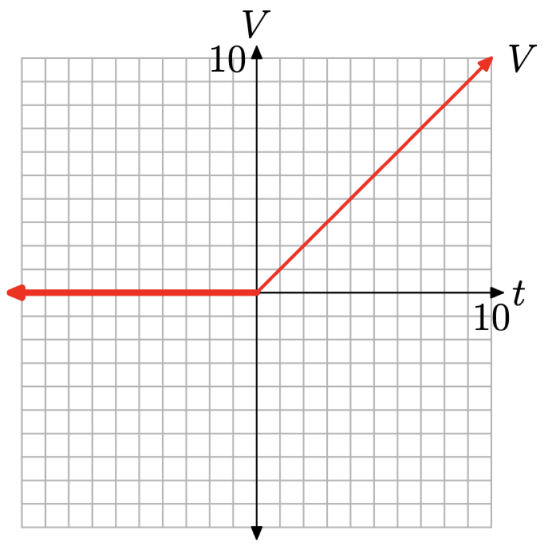
A source provides voltage to a circuit according to the piecewise definition
\[V(t)=\left\{\begin{array}{ll}{0,} & {\text { if } t<0} \\ {t,} & {\text { if } t \geq 0}\end{array}\right. \nonumber \]
Sketch the graph of the voltage V versus time t.
Solution
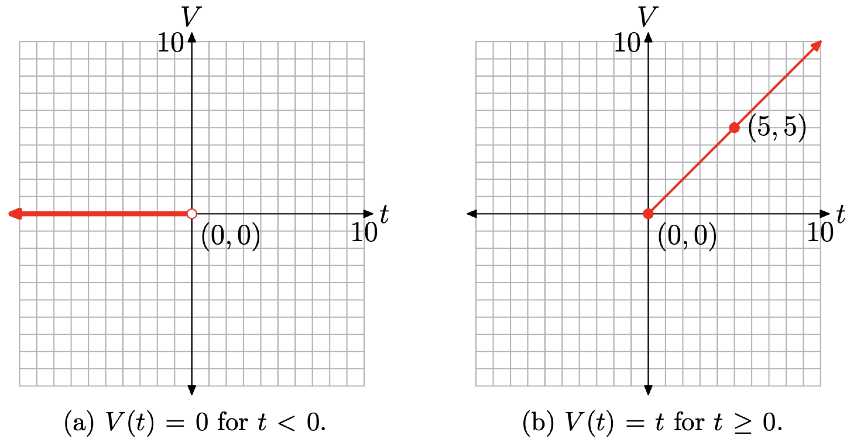
For all time t that is less than zero, the voltage V is zero. The graph of V (t) = 0 is a constant function, so its graph is normally a horizontal line. However, we must restrict
the graph to the domain \((-\infty, 0)\), so this piece of equation (10) will be a horizontal ray, starting at the origin and moving indefinitely to the left, as shown in Figure \(\PageIndex{8}\)(a).
On the other hand, V (t) = t for all values of t that are greater than or equal to zero. Normally, this would be a line with slope 1 and intercept zero. However, we must restrict the domain to \([0, \infty)\), so this piece of equation (10) will be a ray, starting at the origin and moving indefinitely to the right.
- The endpoint of this ray starts at t = 0. Because V (t) = t, V (0) = 0. Hence, the endpoint of this ray is at the point (0, 0).
- Choose any value of t that is greater than zero. We’ll choose t = 5. Because V (t) = t, V (5) = 5. This gives us a second point on the ray at (5, 5), as shown in Figure \(\PageIndex{8}\)(b).
Finally, to provide a complete graph of the voltage function defined by equation (10), we combine the graphs of each piece of the definition shown in Figures \(\PageIndex{8}\)(a) and (b).
The result is shown in Figure \(\PageIndex{9}\). Engineers refer to this type of input function as a “ramp function.”
Let’s look at a very practical application of piecewise functions.
The federal income tax rates for a single filer in the year 2005 are given in Table \(\PageIndex{1}\).
| Income | Tax Rate |
|---|---|
| Up to $7,150 | 10% |
| $7,151-$29,050 | 15% |
| $29,051-$70,350 | 25% |
| $70,351-$146,750 | 28% |
| $146,751-$319,100 | 33% |
| $319,101 or more | 35% |
Create a piecewise definition that provides the tax rate as a function of personal income.
Solution
In reporting taxable income, amounts are rounded to the nearest dollar on the federal income tax form. Technically, the domain is discrete. You can report a taxable income of $35,000 or $35,001, but numbers between these two incomes are not used on the federal income tax form. However, we will think of the income as a continuum, allowing the income to be any real number greater than or equal to zero. If we did not do this, then our graph would be a series of dots–one for each dollar amount. We would have to plot lots of dots!
We will let R represent the tax rate and I represent the income. The goal is to define R as a function of I.
- If income I is any amount greater than or equal to zero, and less than or equal to $7,150, the tax rate R is 10% (i.e., R = 0.10). Thus, if \(\$ 0 \leq I \leq \$ 7,150\), R(I) = 0.10.
- If income I is any amount that is strictly greater than $7,150 but less than or equal to $29,050, then the tax rate R is 15% (i.e., R = 0.15). Thus, if $7, 150 < I ≤ $29, 050, then R(I) = 0.15.
Continuing in this manner, we can construct a piecewise definition of rate R as a function of taxable income I.
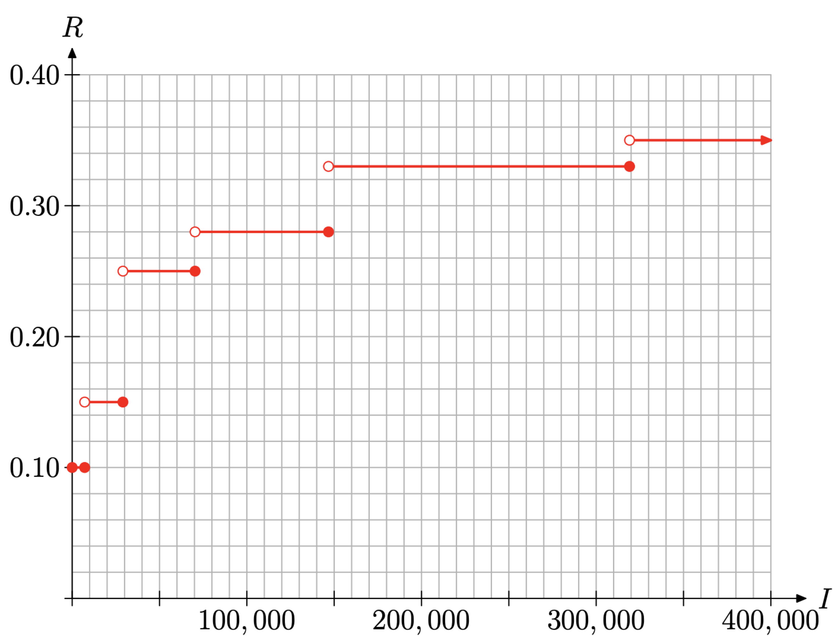
\[R(I)=\left\{\begin{array}{ll}{0.10,} & {\text { if } \$ 0 \leq I \leq \$ 7,150} \\ {0.15,} & {\text { if } \$ 7,150<I \leq \$ 29,050} \\ {0.25,} & {\text { if } \$ 29,050<I \leq \$ 70,350} \\ {0.28,} & {\text { if } \$ 70,350<I \leq \$ 146,750} \\ {0.33,} & {\text { if } \$ 146,750<I \leq \$ 319,100} \\ {0.35,} & {\text { if } I>\$ 319,100}\end{array}\right. \nonumber \]
Let’s turn our attention to the graph of this piecewise-defined function. All of the pieces are constant functions, so each piece will be a horizontal line at a level indicating the tax rate. However, each of the first five pieces of the function defined in equation (12) are segments, because the rate is defined on an interval with a starting and ending income. The sixth and last piece is a ray, as it has a starting endpoint, but the rate remains constant for all incomes above $319,100. We use this knowledge to construct the graph shown in Figure \(\PageIndex{10}\).
The first rate is 10% and this is assigned to taxable income starting at $0 and ending at $7,150, inclusive. Thus, note the first horizontal line segment in Figure \(\PageIndex{10}\) that runs from $0 to $7,150 at a height of R = 0.10. Note that each of the endpoints are filled circles.
The second rate is 15% and this is assigned to taxable incomes greater than $7,150, but less than or equal to $29,050. The second horizontal line segment in Figure 10 runs from $7,150 to $29,050 at a height of R = 0.15. Note that the endpoint at the left end of this horizontal segment is an open circle while the endpoint on the right end is a filled circle because the taxable incomes range on $7, 150 < I ≤ $29, 050. Thus, we exclude the left endpoint and include the right endpoint.
The remaining segments are drawn in a similar manner.
The last piece assigns a rate of R = 0.35 to all taxable incomes strictly above $319,100. Hence, the last piece is a horizontal ray, starting at ($319 100, 0.35) and extending indefinitely to the right. Note that the left endpoint of this ray is an open circle because the rate R = 0.35 applies to taxable incomes I > $319, 100.
Let’s talk a moment about the domain and range of the function R defined by equation (12). The graph of R is depicted in Figure \(\PageIndex{10}\). If we project all points on the graph onto the horizontal axis, the entire axis will “lie in shadow.” Thus, at first
glance, one would state that the domain of R is the set of all real numbers that are greater than or equal to zero.
However, remember that we chose to model a discrete situation with a continuum. Taxable income is always rounded to the nearest dollar on federal income tax forms. Therefore, the domain is actually all whole numbers greater than or equal to zero. In symbols,
\[\text { Domain }=\{I \in \mathbb{W} : I \geq 0\} \nonumber \]
To find the range of R, we would project all points on the graph of R in Figure \(\PageIndex{10}\) onto the vertical axis. The result would be that six points would be shaded on the vertical axis, one each at 0.10, 0.15, 0.25, 0.28, 0.33, and 0.35. Thus, the range is a finite discrete set, so it’s best described by simply listing its members.
\[\text { Range }=\{0.10,0.15,0.25,0.28,0.33,0.35\} \nonumber \]
Exercise
Given the function defined by the rule f(x) = 3, evaluate f(−3), f(0) and f(4), then sketch the graph of f.
- Answer
-
f(−3) = 3, f(0) = 3, and f(4) = 3.
Given the function defined by the rule g(x) = 2, evaluate g(−2), g(0) and g(4), then draw the draw the graph of g.
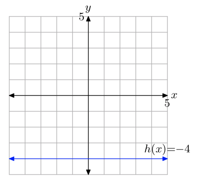
Given the function defined by the rule h(x) = −4, evaluate h(−2), h(a), and h(2x+3), then draw the graph of h.
- Answer
-
h(−2) = −4, h(a) = −4, and h(2x+3) = −4.
Given the function defined by the rule f(x) = −2, evaluate f(0), f(b), and f(5−4x), then draw the graph of f.
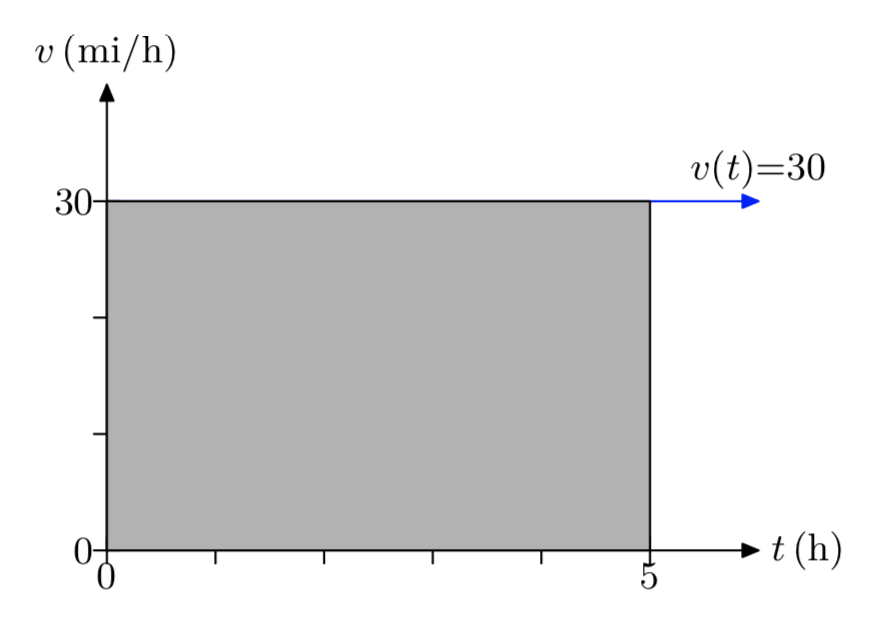
The speed of an automobile traveling on the highway is a function of time and is described by the constant function v(t) = 30, where t is measured in hours and v is measured in miles per hour. Draw the graph of v versus t. Be sure to label each axis with the appropriate units. Shade the area under the graph of v over the time interval [0,5] hours. What is the area under the graph of v over this time interval and what does it represent?
- Answer
-
The area under the curve is 150 miles. This is the distance traveled by the car.
The speed of a skateboarder as she travels down a slope is a function of time and is described by the constant function v(t) = 8, where t is measured in seconds and v is measured in feet per second. Draw the graph of v versus t. Be sure to label each axis with the appropriate units. Shade the area under the graph of v over the time interval [0,60] seconds. What is the area under the graph of v over this time interval and what does it represent?
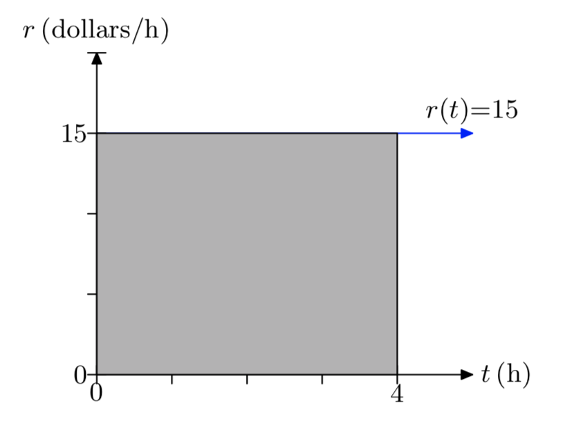
An unlicensed plumber charges 15 dollars for each hour of labor. Let’s define this rate as a function of time by r(t) = 15, where t is measured in hours and r is measured in dollars per hour. Draw the graph of r versus t. Be sure to label each axis with appropriate units. Shade the area under the graph of r over the time interval [0,4] hours. What is area under the graph of r over this time interval and what does it represent?
- Answer
-
The area under the curve is 150 miles. This is the distance traveled by the car.
A carpenter charges a fixed rate for each hour of labor. Let’s describe this rate as a function of time by r(t) = 25, where t is measured in hours and r is measured in dollars per hour. Draw the graph of r versus t. Be sure to label each axis with appropriate units. Shade the area under the graph of r over the time interval [0, 5] hours. What is the area under the graph of r over this time interval and what does it represent?
Given the function defined by the rule
\[f(x)=\left\{\begin{array}{ll}{0,} & {\text { if } x<0} \\ {2,} & {\text { if } x \ge 0} \nonumber \end{array}\right. \nonumber \]
evaluate f(−2), f(0), and f(3), then draw the graph of f on a sheet of graph paper. State the domain and range of f.
- Answer
-
f(−2) = 0, f(0) = 2, and f(3) = 2.
The domain of f is the set of all real numbers. The range of f is {0, 2}.
Given the function defined by the rule
\[f(x)=\left\{\begin{array}{ll}{2,} & {\text { if } x<0} \\ {0,} & {\text { if } x \ge 0} \nonumber \end{array}\right. \nonumber \]
evaluate f(−2), f(0), and f(3), then draw the graph of f on a sheet of graph paper. State the domain and range of f.
Given the function defined by the rule
\[f(x)=\left\{\begin{array}{ll}{-3,} & {\text { if } x<0} \\ {1,} & {\text { if } -2 \le x < 2}\\ {3,} &{\text{ if } x \ge 2} \nonumber \end{array}\right. \nonumber \]
evaluate g(−3), g(−2), and g(5), then draw the graph of g on a sheet of graph paper. State the domain and range of g.
- Answer
-
g(−3) = −3, g(−2) = 1, and g(5) = 3
The domain of g is all real numbers. The range of g is {−3, 1, 3}.
Given the function defined by the rule
\[f(x)=\left\{\begin{array}{ll}{4,} & {\text { if } x \le -1} \\ {2,} & {\text { if } -1 < x \le 2}\\ {-3,} &{\text{ if } x > 2} \nonumber \end{array}\right. \nonumber \]
evaluate g(−1), g(2), and g(3), then draw the graph of g on a sheet of graph paper. State the domain and range of g.
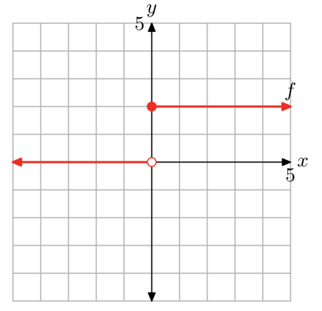
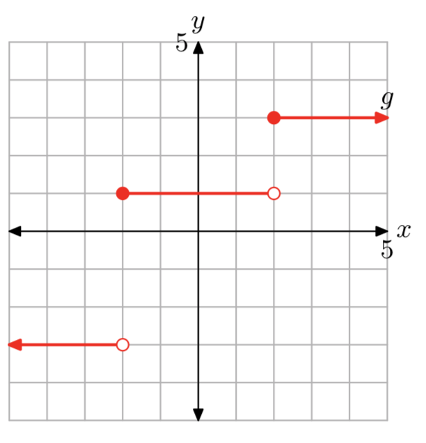
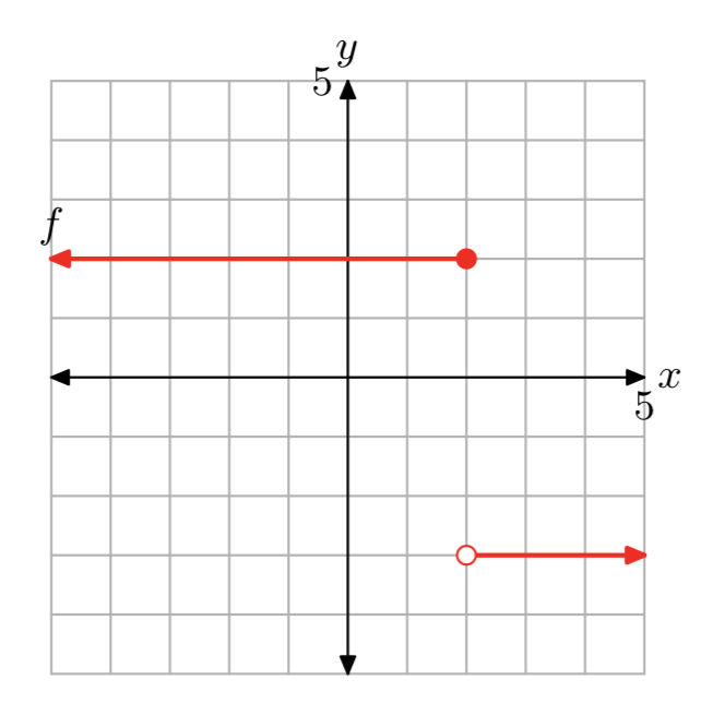
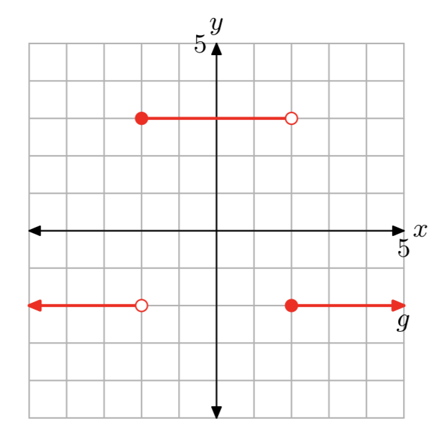
In Exercises 13-16, determine a piecewise definition of the function described by the graphs, then state the domain and range of the function.
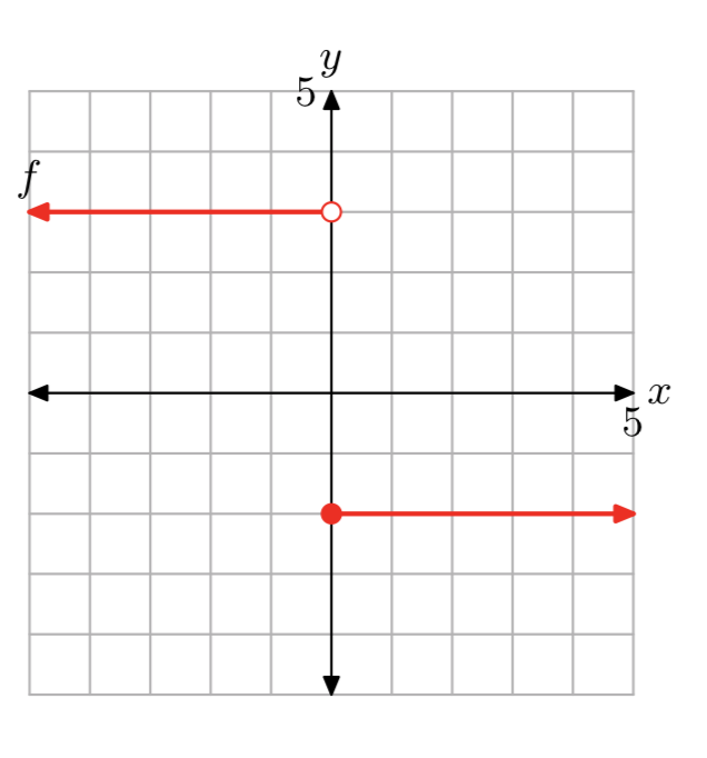
- Answer
-
\[f(x)=\left\{\begin{array}{ll}{3,} & {\text { if } x<0} \\ {-2,} & {\text { if } x \ge 0} \nonumber \end{array}\right. \nonumber \]
Domain of f is the set of all real numbers. The range of f is {−2, 3}.
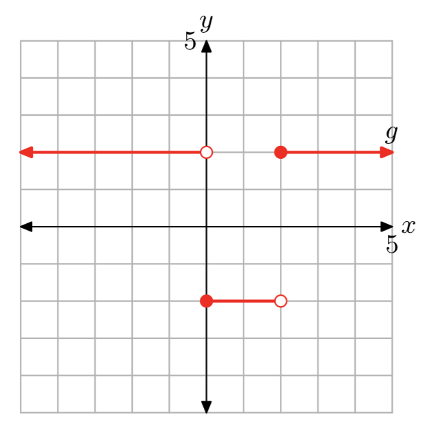
- Answer
-
\[g(x)=\left\{\begin{array}{ll}{2,} & {\text { if } x < 0} \\ {-2,} & {\text { if } 0 \le x < 2}\\ {2,} &{\text{ if } x > 2} \nonumber \end{array}\right. \nonumber \]
The domain of f is the set of all real numbers. The range of f is {−2, 2}.
Given the piecewise function
\[f(x)=\left\{\begin{array}{ll}{-x-3,} & {\text { if } x<-3} \\ {x+3,} & {\text { if } x \ge -3} \nonumber \end{array}\right. \nonumber \]
evaluate f(−4) and f(0), then draw the graph of f on a sheet of graph paper. State the domain and range of the function.
- Answer
-
f(−4) = 1 and f(0) = 3.
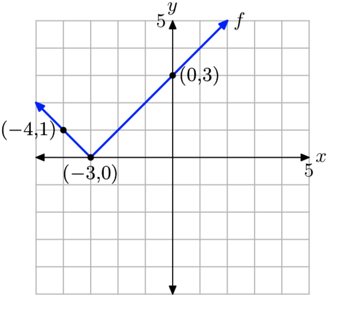
The domain of f is the set of all real numbers. The range off is{y: \(y \ge 0\)}.
Given the piecewise function
\[f(x)=\left\{\begin{array}{ll}{-x+1,} & {\text { if } x<1} \\ {x-1,} & {\text { if } x \ge 1} \nonumber \end{array}\right. \nonumber \]
evaluate f(−2) and f(3), then draw the graph of f on a sheet of graph paper. State the domain and range of the function.
Given the piecewise function
\[g(x)=\left\{\begin{array}{ll}{-2x+3,} & {\text { if } x<\frac{3}{2}} \\ {2x-3,} & {\text { if } x \ge \frac{3}{2}} \nonumber \end{array}\right. \nonumber \]
evaluate g(0) and g(3), then draw the graph of f on a sheet of graph paper. State the domain and range of the function.
- Answer
-
g(−2) = 7 and g(2) = 1.
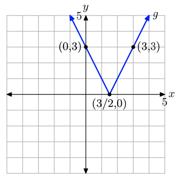
The domain of g is the set of all real numbers. The range off is{y: \(y \ge 0\)}.
Given the piecewise function
\[g(x)=\left\{\begin{array}{ll}{-3x-4,} & {\text { if } x<-\frac{4}{3}} \\ {3x+4,} & {\text { if } x \ge -\frac{4}{3}} \nonumber \end{array}\right. \nonumber \]
evaluate g(−2) and g(3), then draw the graph of f on a sheet of graph paper. State the domain and range of the function.
A battery supplies voltage to an electric circuit in the following manner. Before time t = 0 seconds, a switch is open, so the voltage supplied by the battery is zero volts. At time t = 0 seconds, the switch is closed and the battery begins to supply a constant 3 volts to the circuit. At time t = 2 seconds, the switch is opened again, and the voltage supplied by the battery drops immediately to zero volts. Sketch a graph of the voltage vversus time t, label each axis with the appropriate units, then provide a piecewise definition of the voltage v supplied by the battery as a function of time t.
- Answer
-
The graph follows.
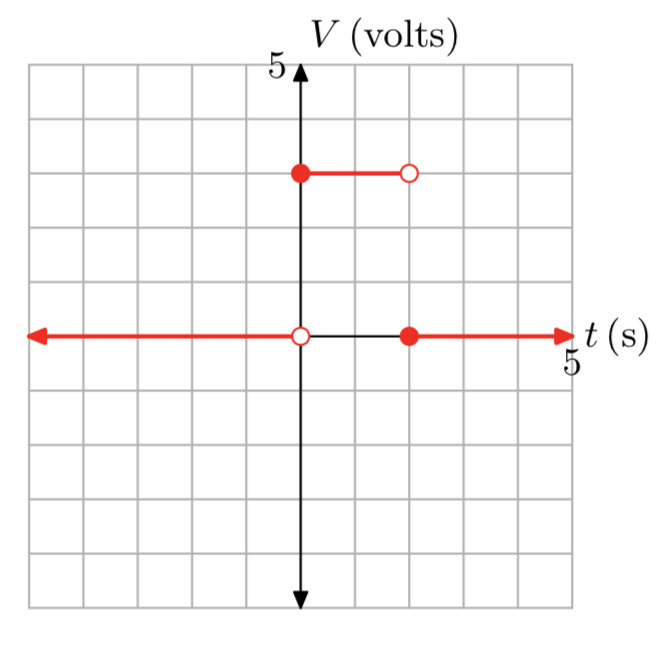
\[g(x)=\left\{\begin{array}{ll}{0,} & {\text { if } x<0} \\ {3,} & {\text { if } 0 \le x < 2}\\ {0,} & {\text{ if } x \ge 2} \nonumber \end{array}\right. \nonumber \]
Prior to time t = 0 minutes, a drum is empty. At time t = 0 minutes a hose is turned on and the water level in the drum begins to rise at a constant rate of 2 inches every minute. Let h represent water level (in inches) at time t (in minutes). Sketch the graph of h versust, label the axes with appropriate units, then provide a piecewise definition of has a function of t.