5.3: 5.3 Cobweb Plots for One-Dimensional Iterative Maps


( \newcommand{\kernel}{\mathrm{null}\,}\)
One possible way to solve the overcrowded phase space of a discrete-time system is to create two phase spaces, one for time t−1 and another for t, and then draw trajectories of the system’s state in a meta-phase space that is obtained by placing those two phase spaces orthogonally to each other. In this way, you would potentially disentangle the tangled trajectories to make them visually understandable.
However, this seemingly brilliant idea has one fundamental problem. It works only for one-dimensional systems, because two- or higher dimensional systems require fouror more dimensions to visualize the meta-phase space, which can’t be visualized in the three-dimensional physical world in which we are confined.
This meta-phase space idea is still effective and powerful for visualizing the dynamics of one-dimensional iterative maps. The resulting visualization is called a cobweb plot, which plays an important role as an intuitive analytical tool to understand the nonlinear dynamics of one-dimensional systems.
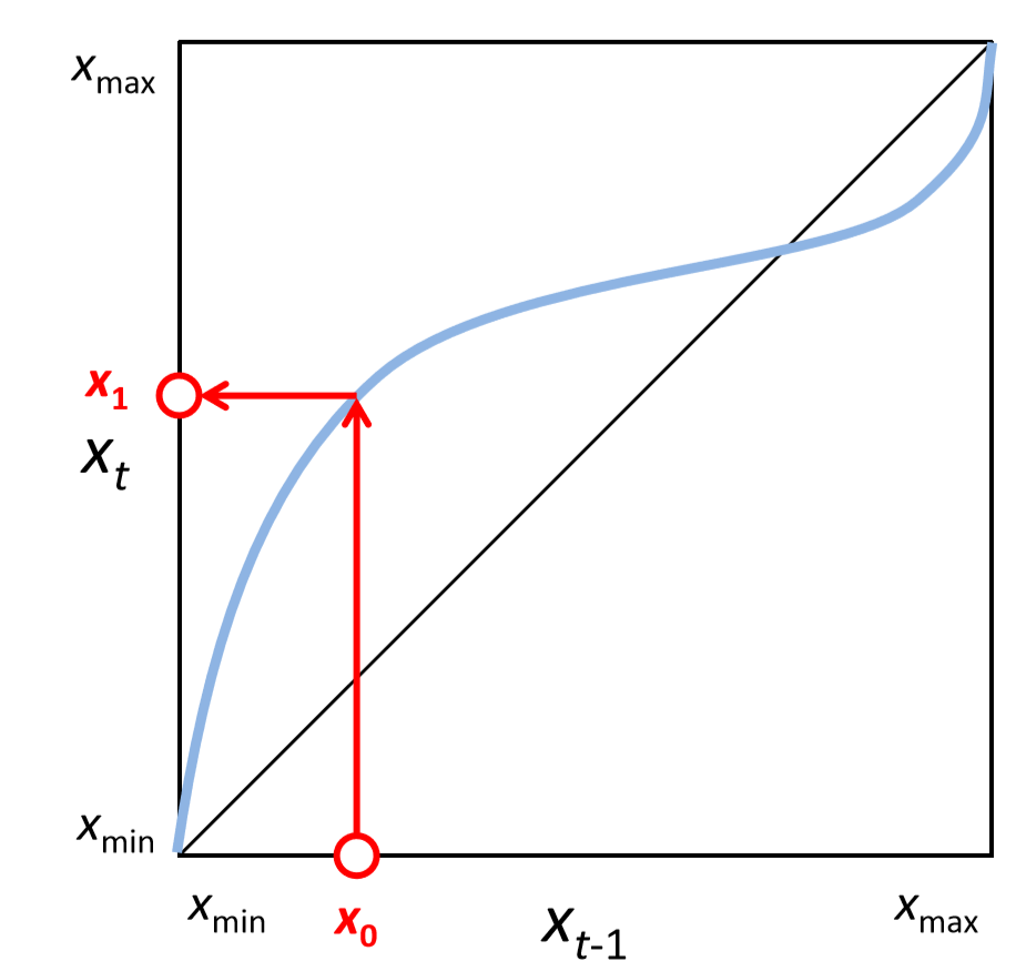
Here is how to manually draw a cobweb plot of a one-dimensional iterative map, xt=f(xt−1), with the range of xt being [xmin,xmax]. Get a piece of paper and a pen, and do the following:
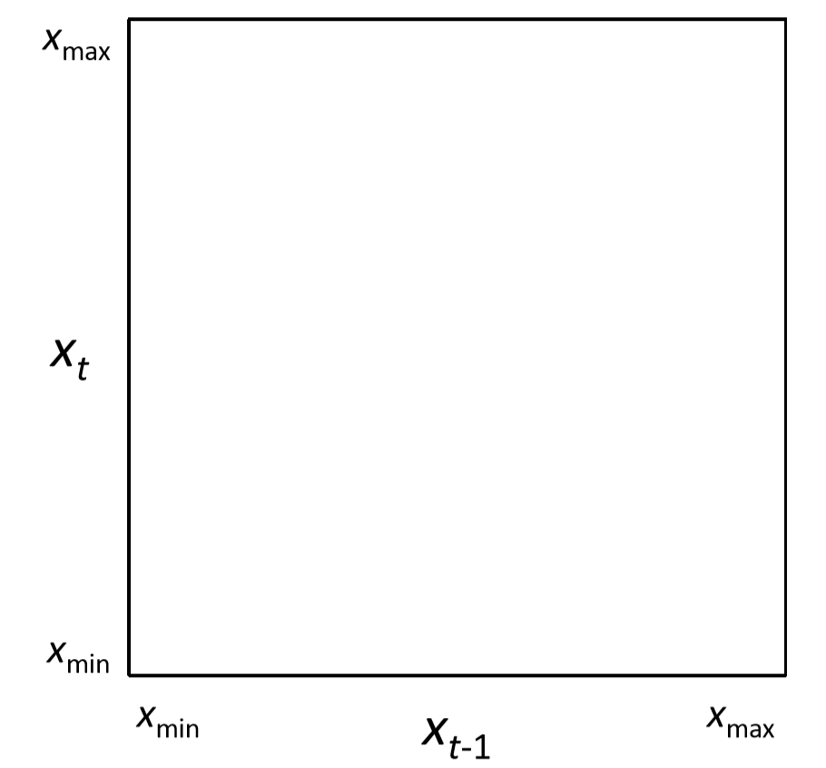
1. Draw a square on your paper. Label the bottom edge as the axis for xt−1, and the left edge as the axis for xt. Label the range of their values on the axes (Fig. 5.3.1).
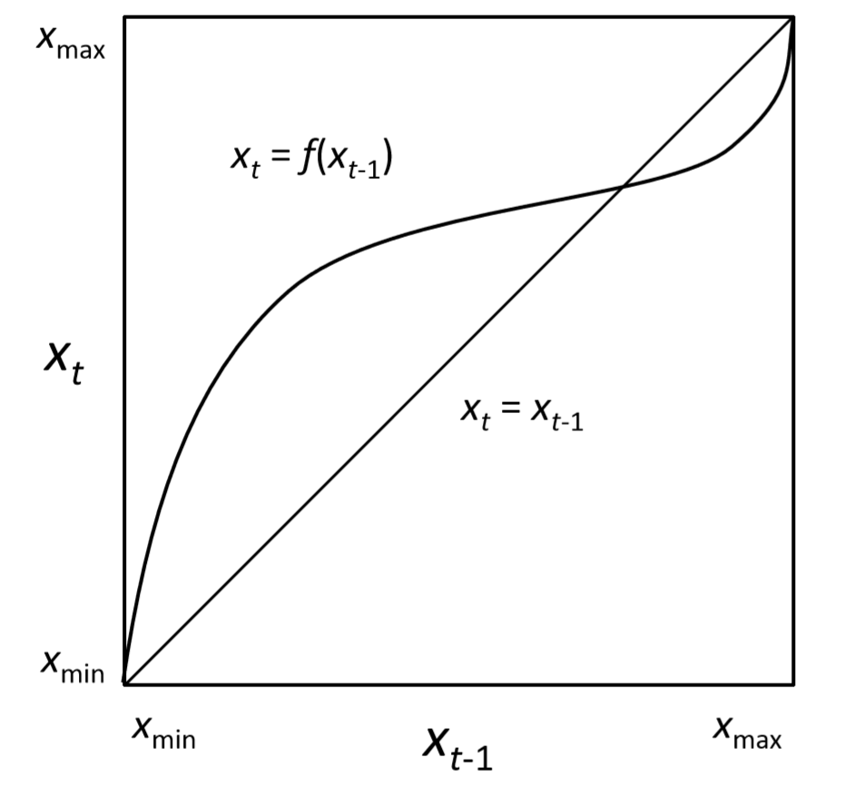
2. Draw a curve xt=f(xt−1) and a diagonal line xt=xt−1 within the square (Fig. 5.3.2). Note that the system’s equilibrium points appear in this plot as the points where the curve and the line intersect.
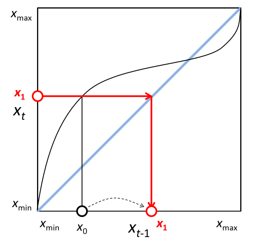
3. Draw a trajectory from xt−1 to xt. This can be done by using the curve xt=f(xt−1) (Fig. 5.3.3). Start from a current state value on the bottom axis (initially, this is the initial value x0, as shown in Fig. 5.3.3), and move vertically until you reach the curve. Then switch the direction of the movement to horizontal and reach the left axis. You end up at the next value of the system’s state (x1 in Fig. 5.3.3). The two red arrows connecting the two axes represent the trajectory between the two consecutive time points.
4. Reflect the new state value back onto the horizontal axis. This can be done as a simple mirror reflection using the diagonal line (Fig. 5.3.4). This completes one step of the “manual simulation” on the cobweb plot.
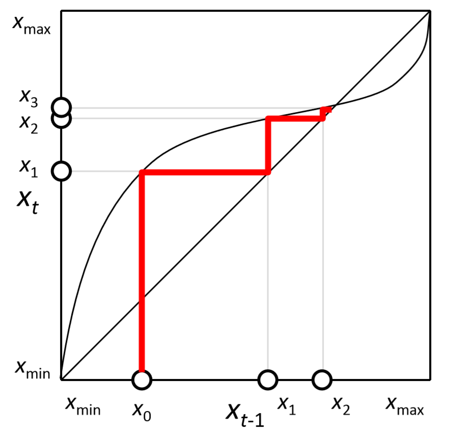
5. Repeat the steps above to see where the system eventually goes (Fig. 5.3.5).
6. Once you get used to this process, you will notice that you don’t really have to touch either axis. All you need to do to draw a cobweb plot is to bounce back and forth between the curve and the line (Fig. 5.3.6)—move vertically to the curve, horizontally to the line, and repeat.
Draw a cobweb plot for each of the following models:
- xt=xt−1+0.1,x0=0.1
- xt=1.1xt−1,x0=0.1
Draw a cobweb plot of the following logistic growth model with r=1,K=1, N0=0.1:
Nt=Nt−1+rNt−1(1−Nt−1K)
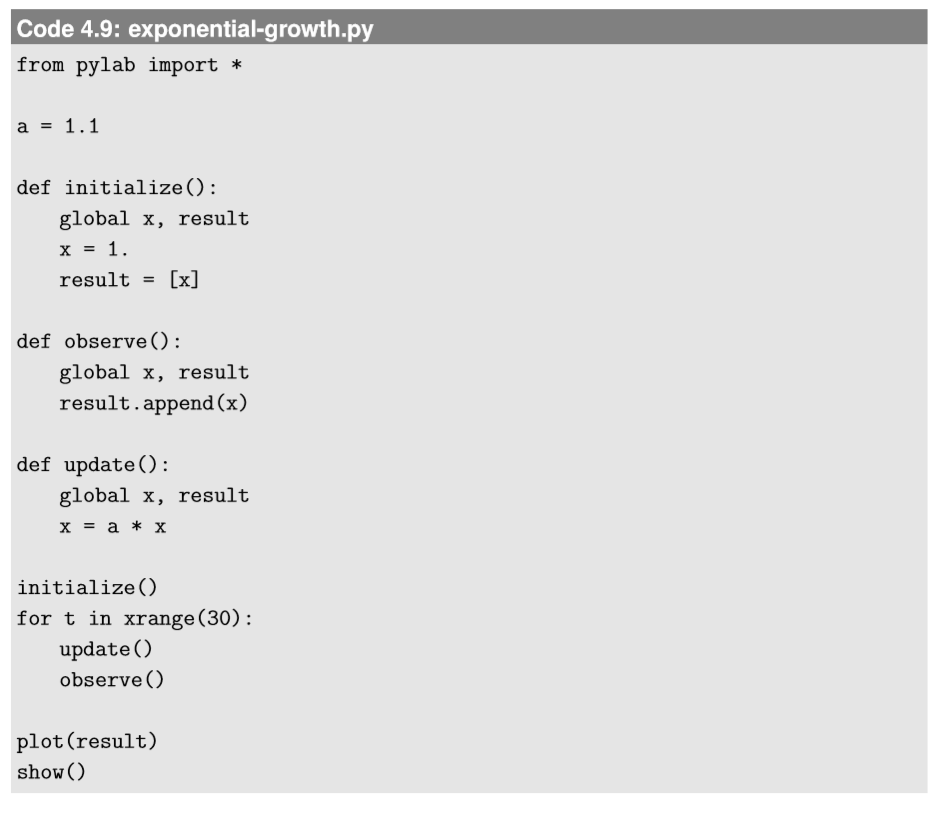
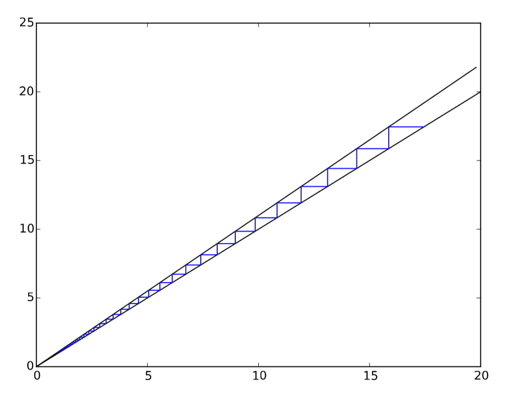
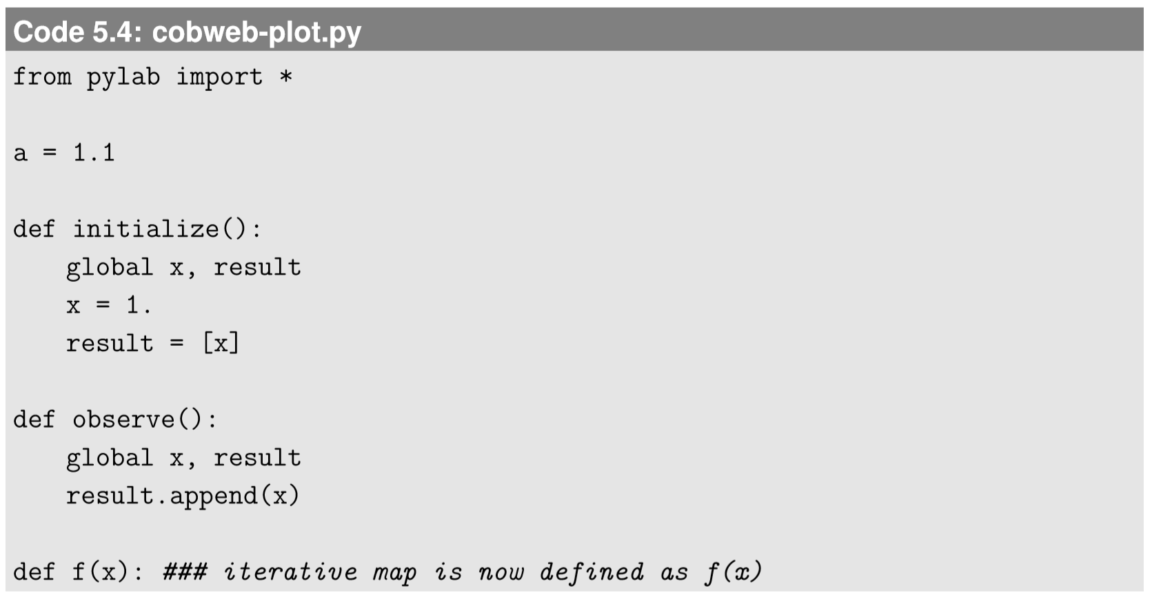
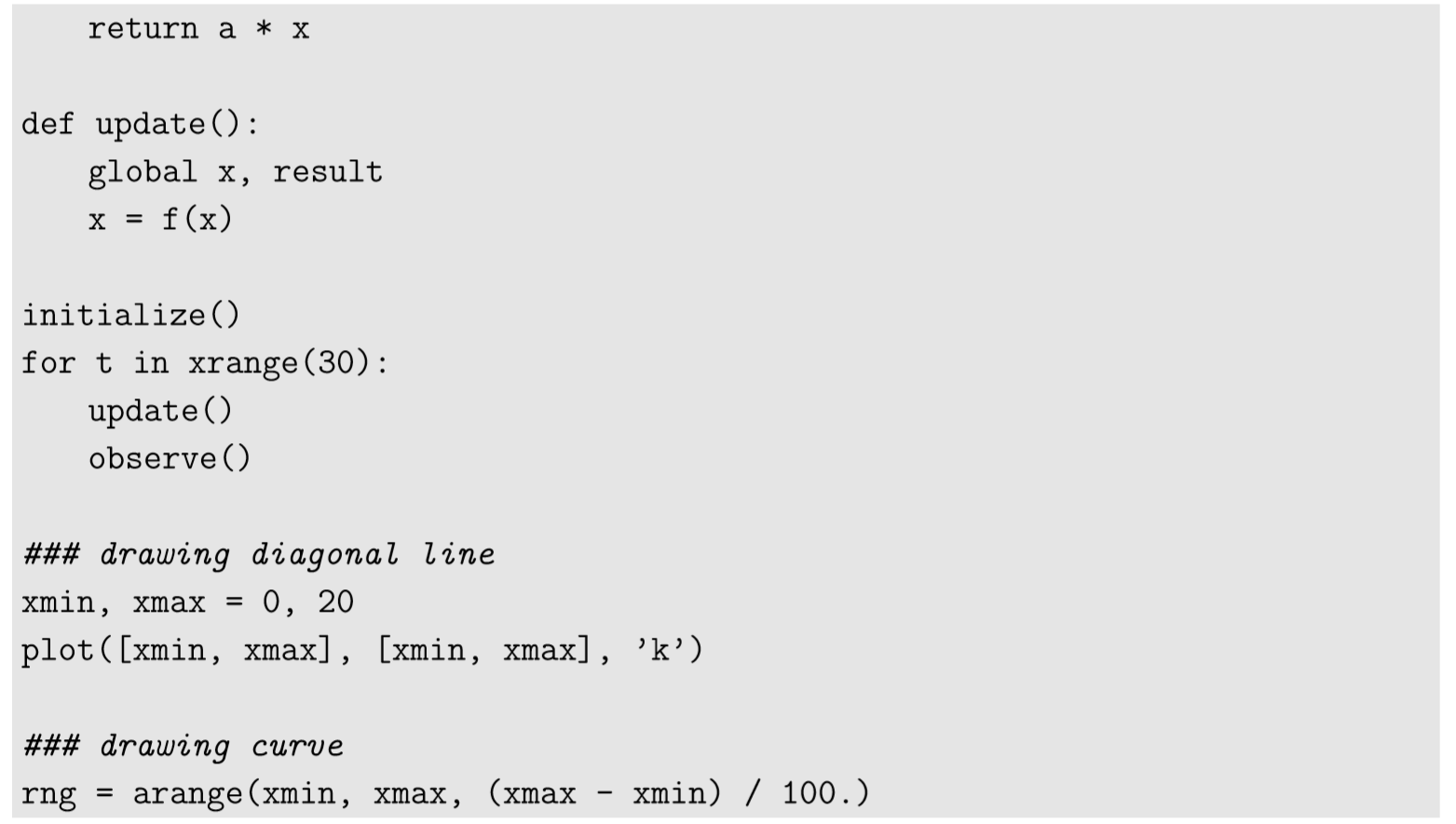
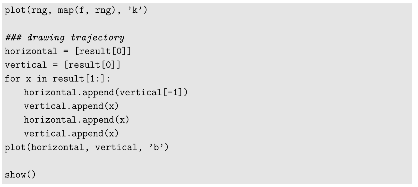
Cobweb plots can also be drawn using Python. Code 5.4 is an example of how to draw a cobweb plot of the exponential growth model (Code 4.9). Its output is given in Fig. 5.4.1.

Using Python, draw a cobweb plot of the logistic growth model with r=2.5, K=1, N0=0.1.