17.6: Assortativity

Degrees are a metric measured on individual nodes. But when we focus on the edges, there are always two degrees associated with each edge, one for the node where the edge originates and the other for the node to where the edge points. So if we take the former for x and the latter for y from all the edges in the network, we can produce a scatter plot that visualizes a possible degree correlation between the nodes across the edges. Such correlations of node properties across edges can be generally described with the concept of assortativity:

Assortativity (positive assortativity) The tendency for nodes to connect to other nodes with similar properties within a network.
Disassortativity (negative assortativity) The tendency for nodes to connect to other nodes with dissimilar properties within a network.

Assortativity coefficient

\[r =\frac{ \sum_{(i,j)\epsilon{E}}(f(i) -\bar{f} _{1})(f(j) -\bar{f}_{2})}{ \sqrt{\sum_{(i,j)\epsilon{E}} (f(j) -\bar{f}_{2}) } \sqrt{ \sum_{(i,j)\epsilon{E}} (f(j) -\bar{f}_{2})^{2}} } \label{(17.33)} \]

where \(E\) is the set of directed edges (undirected edges should appear twice in \(E\) in two directions), and
\[\bar{f}_{1} =\frac{\sum_{i,j}\epsilon{E} {f(i)}}{|E|}, \qquad \bar{f}_{2} =\frac{\sum_{i,j}\epsilon{E} f(j)}{|E|}. \label{(17.34)} \]

The assortativity coefficient is a Pearson correlation coefficient of some node property \(f\) between pairs of connected nodes. Positive coefficients imply assortativity, while negative ones imply disassortativity.

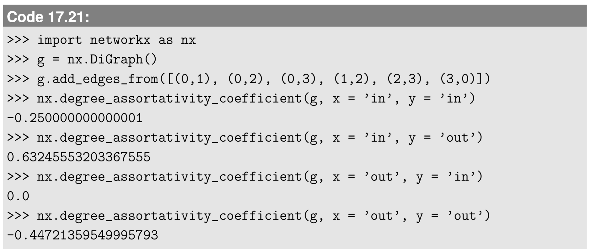
If the measured property is a node degree (i.e., \(f = deg\)), this is called the degree assortativity coefficient. For directed networks, each of \(\bar{f}_1\) an \(\bar{f}_2\) can be either in-degree or out-degree, so there are four different degree assortativities you can measure: in-in, in-out, out-in, and out-out.

Let’s look at some example. Here is how to draw a degree-degree scatter plot:

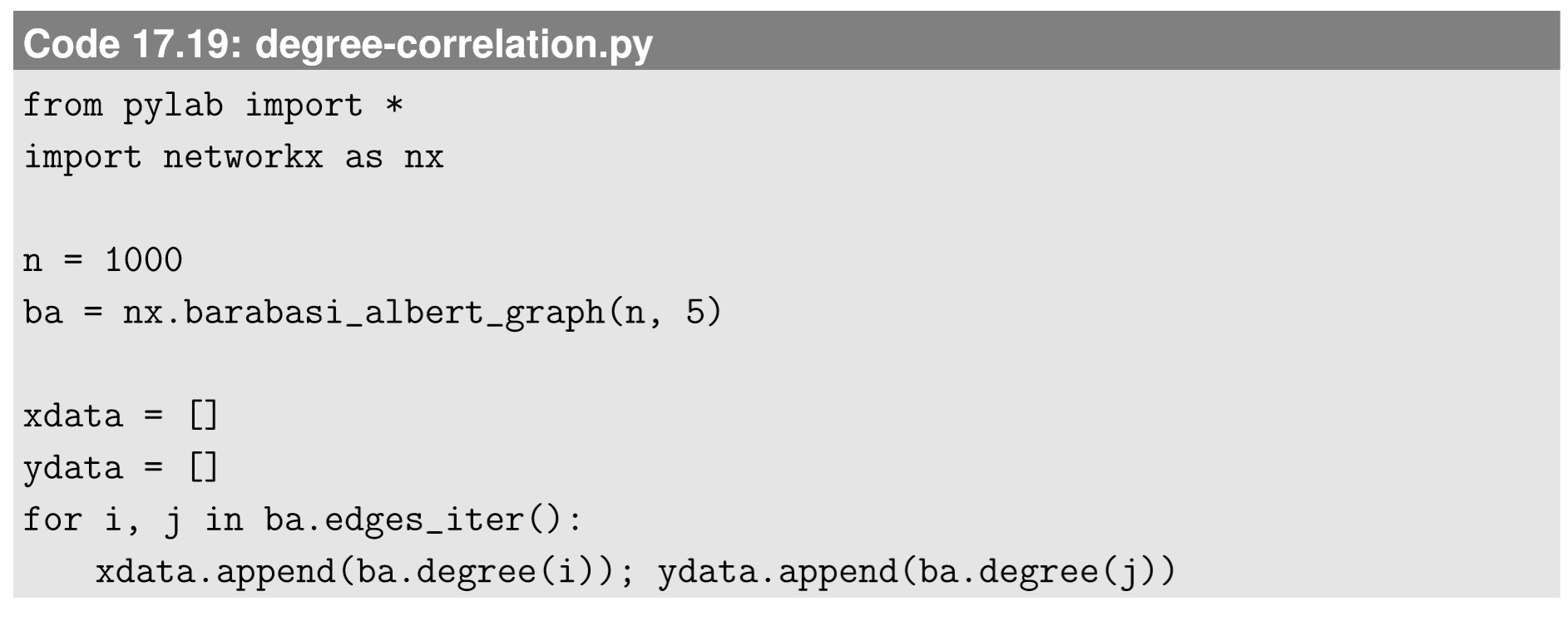
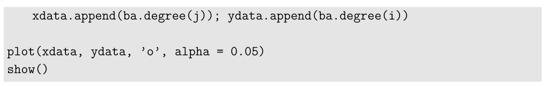
In this example, we draw a degree-degree scatter plot for a Barab´asi-Albert network with 1,000 nodes. For each edge, the degrees of its two ends are stored in xdata and ydata twice in different orders, because an undirected edge can be counted in two directions. The markers in the plot are made transparent using the alpha option so that we can see the density variations in the plot.

The result is shown in Fig. 17.6.1, where each dot represents one directed edge in the network (so, an undirected edge is represented by two dots symmetrically placed across a diagonal mirror line). It can be seen that most edges connect low-degree nodes to each other, with some edges connecting low-degree and high-degree nodes, but it is quite rare that high-degree nodes are connected to each other. Therefore, there is a mild negative degree correlation in this case.

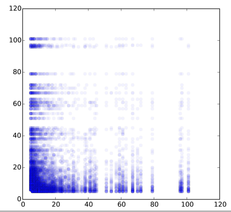
Figure \(\PageIndex{1}\): Visual output of code 17.19.
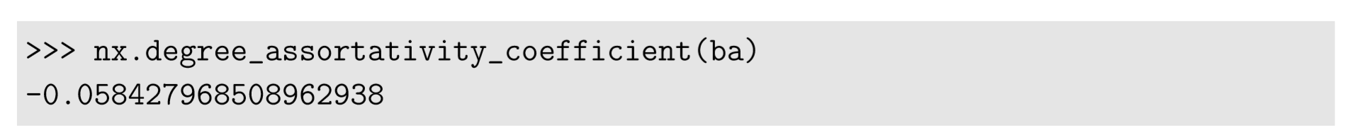
We can confirm this observation by calculating the degree assortativity coefficient as follows:

This function also has options x (for \(\bar{f}_1\)) and y (for \(\bar{f}_2\)) to specify which degrees you use in calculating coefficients for directed networks:

There are also other functions that can calculate assortativities of node properties other than degrees. Check out NetworkX’s online documentation for more details.

Exercise \(\PageIndex{1}\)

Measure the degree assortativity coefficient of the Karate Club graph. Explain the result in view of the actual topology of the graph.

It is known that real-world networks show a variety of assortativity. In general, social networks of human individuals, such as collaborative relationships among scientists or corporate directors, tend to show positive assortativity, while technological networks (power grid, the Internet, etc.) and biological networks (protein interactions, neural networks, food webs, etc.) tend to show negative assortativity [76].

In the meantime, it is also known that scale-free networks of a finite size (which many real-world networks are) naturally show negative disassortativity purely because of inherent structural limitations, which is called a structural cutoff [25]. Such disassortativity arises because there are simply not enough hub nodes available for themselves to connect to each other to maintain assortativity. This means that the positive assortativities found in human social networks indicate there is definitely some assortative mechanism driving their self-organization, while the negative assortativities found in technological and biological networks may be explained by this simple structural reason. In order to determine whether or not a network showing negative assortativity is fundamentally disassortative for non-structural reasons, you will need to conduct a control experiment by randomizing its topology and measuring assortativity while keeping the same degree distribution.

Exercise \(\PageIndex{2}\)

Randomize the topology of the Karate Club graph while keeping its degree sequence, and then measure the degree assortativity coefficient of the randomized graph. Repeat this many times to obtain a distribution of the coefficients for randomized graphs. Then compare the distribution with the actual assortativity of the original Karate Club graph. Based on the result, determine whether or not the Karate Club graph is truly assortative or disassortative.