7.3: Euler's Method

Last updated
Save as PDF

Page ID: 4336

$ \newcommand{\vecs}[1]{\overset { \scriptstyle \rightharpoonup} {\mathbf{#1}} } $ $ \newcommand{\vecd}[1]{\overset{-\!-\!\rightharpoonup}{\vphantom{a}\smash {#1}}} $$\newcommand{\id}{\mathrm{id}}$ $ \newcommand{\Span}{\mathrm{span}}$ $ \newcommand{\kernel}{\mathrm{null}\,}$ $ \newcommand{\range}{\mathrm{range}\,}$ $ \newcommand{\RealPart}{\mathrm{Re}}$ $ \newcommand{\ImaginaryPart}{\mathrm{Im}}$ $ \newcommand{\Argument}{\mathrm{Arg}}$ $ \newcommand{\norm}[1]{\| #1 \|}$ $ \newcommand{\inner}[2]{\langle #1, #2 \rangle}$ $ \newcommand{\Span}{\mathrm{span}}$ $\newcommand{\id}{\mathrm{id}}$ $ \newcommand{\Span}{\mathrm{span}}$ $ \newcommand{\kernel}{\mathrm{null}\,}$ $ \newcommand{\range}{\mathrm{range}\,}$ $ \newcommand{\RealPart}{\mathrm{Re}}$ $ \newcommand{\ImaginaryPart}{\mathrm{Im}}$ $ \newcommand{\Argument}{\mathrm{Arg}}$ $ \newcommand{\norm}[1]{\| #1 \|}$ $ \newcommand{\inner}[2]{\langle #1, #2 \rangle}$ $ \newcommand{\Span}{\mathrm{span}}$$\newcommand{\AA}{\unicode[.8,0]{x212B}}$

Learning Objectives

In this section, we strive to understand the ideas generated by the following important questions:

What is Euler’s method and how can we use it to approximate the solution to an initial value problem?
How accurate is Euler’s method?

In Section 7.2, we saw how a slope field can be used to sketch solutions to a differential equation. In particular, the slope field is a plot of a large collection of tangent lines to a large number of solutions of the differential equation, and we sketch a single solution by simply following these tangent lines. With a little more thought, we may use this same idea to numerically approximate the solutions of a differential equation.

Preview Activity $\PageIndex{1}$

Consider the initial value problem

$\dfrac{dy}{ dt} = \dfrac{1}{ 2 (y + 1)}$

with $y(0) = 0$.

Use the differential equation to find the slope of the tangent line to the solution $y(t)$ at $t = 0$. Then use the given initial value to find the equation of the tangent line at $t = 0$.
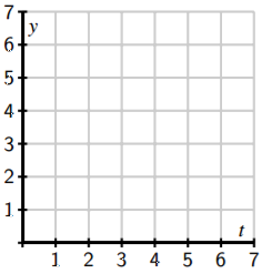
Sketch the tangent line on the axes below on the interval $0 ≤ t ≤ 2$ and use it to approximate $y(2)$, the value of the solution at $t = 2$.
Assuming that your approximation for $y(2)$ is the actual value of $y(2)$, use the differential equation to find the slope of the tangent line to $y(t)$ at $t = 2$. Then, write the equation of the tangent line at $t = 2$.
Add a sketch of this tangent line to your plot on the axes above on the interval $2 \leq t \leq 4$; use this new tangent line to approximate $y(4)$, the value of the solution at $t = 4$.
Repeat the same step to find an approximation for $y(6)$.

$alt$

Euler’s Method

Preview Activity $\PageIndex{1}$ demonstrates the essence of an algorithm, which is known as Euler’s Method, that generates a numerical approximation to the solution of an initial value problem. In this algorithm, we will approximate the solution by taking horizontal steps of a fixed size that we denote by $\Delta t$.

Before explaining the algorithm in detail, let’s remember how we compute the slope of a line: the slope is the ratio of the vertical change to the horizontal change, as shown in the following figure.

$alt$

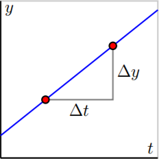
In other words, $m = \frac{\Delta y}{\Delta t}$. Said differently, the vertical change is the product of the slope and the horizontal change:

$\Delta y = m\Delta t.$

Suppose that we would like to solve the initial value problem

$\dfrac{dy}{dt} = t − y, y(0) = 1.$

“Euler” is pronounced “Oy-ler.” Among other things, Euler is the mathematician credited with the famous number e; if you incorrectly pronounce his name “You-ler,” you fail to appreciate his genius and legacy.

While there is an algorithm by which we can find an algebraic formula for the solution to this initial value problem, and we can check that this solution is

$y(t) = t − 1 + 2e^{ −t},$

we are instead interested in generating an approximate solution by creating a sequence of points $(t_i , y_i)$, where $y_i \approx y(t_i)$. For this first example, we choose $\Delta t = 0.2$. Since we know that $y(0) = 1$, we will take the initial point to be $(t_0, y_0) = (0, 1)$ and move horizontally by $\Delta t = 0.2$ to the point $(t_1, y_1)$. Therefore,

$t_1 = t_0 + \Delta t = 0.2.$

The differential equation tells us that the slope of the tangent line at this point is

$m = \left.\dfrac{dy}{ dt}\right|_{(0,1)} = 0 − 1 = −1.$

$alt$

Therefore, if we move along the tangent line by taking a horizontal step of size $\Delta t = 0.2$, we must also move vertically by

$\Delta y = m\Delta t = −1 · 0.2 = −0.2.$

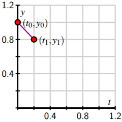
We then have the approximation

$y(0.2) \approx y_1 = y_0 + \Delta y = 1 − 0.2 = 0.8.$

At this point, we have executed one step of Euler’s method. 0.4 0.8 1.2 0.4 0.8 1.2 $(t_0,y_0) (t_1,y_1) t y$ Now we repeat this process: at $(t_1, y_1) = (0.2, 0.8)$, the differential equation tells us that the slope is $m = dy/dt (0.2,0.8) = 0.2 − 0.8 = −0.6$.

$alt$

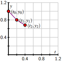
If we move horizontally by $\Delta t$ to $t_2 = t_1 +\Delta = 0.4$, we must move vertically by

$\Delta y = −0.6 · 0.2 = −0.12.$

We consequently arrive at $y_2 = y_1+\Delta y = 0.8−0.12 = 0.68,$ which gives $y(0.2) \approx 0.68$. Now we have completed the second step of Euler’s method.

If we continue in this way, we may generate the points $(t_i , y_i)$ shown at left in Figure $\PageIndex{1}$. In situations where we are able to find a formula for the actual solution $ y(t)$, we can graph $ y(t)$ to compare it to the points generated by Euler’s method, as shown at right in Figure $\PageIndex{1}$.

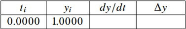
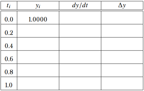
Because we need to generate a large number of points $(t_i , y_i)$, it is convenient to organize the implementation of Euler’s method in a table as shown. We begin with the given initial data.

$alt$

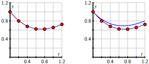
Figure $\PageIndex{1}$: At left, the points and piecewise linear approximate solution generated by Euler’s method; at right, the approximate solution compared to the exact solution (shown in blue).

$alt$

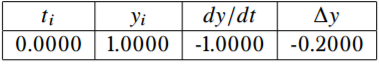
From here, we compute the slope of the tangent line $m = dy/dt$ using the formula for $dy/dt$ from the differential equation, and then we find $\Delta y$, the change in $y$, using the rule $\Delta y=m\Delta t$.

$alt$

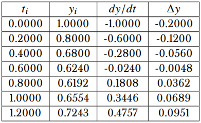
Next, we increase $t_i$ by $\Delta t$ and $y_i$ by $\Delta y$ to get

$alt$

and then we simply continue the process for however many steps we decide, eventually generating a table like the one that follows.

$alt$

Activity $\PageIndex{1}$

Consider the initial value problem

$\dfrac{dy}{dt} = 2t − 1,\ y(0) = 0$

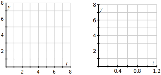
(a) Use Euler’s method with $\Delta t = 0.2$ to approximate the solution at $t_i = 0.2$, $0.4$, $0.6$, $0.8$, and $1.0$. Record your work in the following table, and sketch the points $(t_i , y_i)$ on the following axes provided.

$alt$

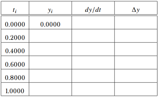
Find the exact solution to the original initial value problem and use this function to find the error in your approximation at each one of the points $t_i$.
Explain why the value $y_5$ generated by Euler’s method for this initial value problem produces the same value as a left Riemann sum for the definite integral $\int^1_0 (2t − 1) \,dt.$
How would your computations differ if the initial value were $y(0) = 1$ instead? What does this mean about different solutions to this differential equation?

Exercise $\PageIndex{2}$

Consider the differential equation

$\dfrac{dy}{dt} = 6y − y^2 .$

Sketch the slope field for this differential equation on the axes provided at left below.
Identify any equilibrium solutions and determine whether they are stable or unstable.
What is the long-term behavior of the solution that satisfies the initial value $y(0) = 1$?
Using the initial value $y(0) = 1$, use Euler’s method with $\Delta t = 0.2$ to approximate the solution at $t_i = 0.2$, $0.4$, $0.6$, $0.8$, and $1.0$. Sketch the points $(t_i , y_i)$ on the axes provided at right in (a). (Note the different horizontal scale on the two sets of axes.)
What happens if we apply Euler’s method to approximate the solution with $y(0) = 6$?

$alt$

The Error in Euler’s Method

Since we are approximating the solutions to an initial value problem using tangent lines, we should expect that the error in the approximation will be less when the step size is smaller. To explore this observation quantitatively, let’s consider the initial value problem

$\dfrac{dy}{dt} = y,\ y(0) = 1$

whose solution we can easily find.

Consider the question posed by this initial value problem: “what function do we know that is the same as its own derivative and has value 1 when $t = 0$?” It is not hard to see that the solution is $y(t) = e^t$. We now apply Euler’s method to approximate $y(1) = e$ using several values of $\Delta t$. These approximations will be denoted by $E_{\Delta t}$, and these estimates provide us a way to see how accurate Euler’s Method is.

To begin, we apply Euler’s method with a step size of $\Delta t = 0.2$. In that case, we find that $y(1) \approx E_{0.2} = 2.4883.$ The error is therefore $y(1) − E_{0.2} = e − 2.4883 \approx 0.2300.$

Repeatedly halving $\Delta t$ gives the following results, expressed in both tabular and graphical form.

$alt$

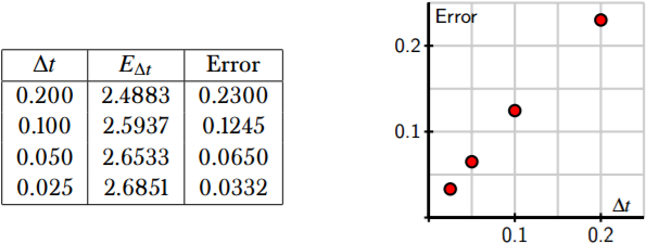
Notice, both numerically and graphically, that the error is roughly halved when $ \Delta t $ is halved. This example illustrates the following general principle.

Euler's Approximation

If Euler’s method is to approximate the solution to an initial value problem at a point $t$, then the error is proportional to $\Delta t$. That is,

$y(\bar{t}) − E_{\Delta t} \approx K\Delta t$

for some constant of proportionality $K$.

Summary

In this section, we encountered the following important ideas:

Euler’s method is an algorithm for approximating the solution to an initial value problem by following the tangent lines while we take horizontal steps across the $t$-axis.
If we wish to approximate $y(\bar{t})$ for some fixed $\bar{t}$ by taking horizontal steps of size $\Delta t$, then the error in our approximation is proportional to $\Delta t$.

Contributors and Attributions

Matt Boelkins (Grand Valley State University), David Austin (Grand Valley State University), Steve Schlicker (Grand Valley State University)