
11.1: Vector–Valued Functions
- Page ID
- 4220

\( \newcommand{\vecs}[1]{\overset { \scriptstyle \rightharpoonup} {\mathbf{#1}} } \)
\( \newcommand{\vecd}[1]{\overset{-\!-\!\rightharpoonup}{\vphantom{a}\smash {#1}}} \)
\( \newcommand{\dsum}{\displaystyle\sum\limits} \)
\( \newcommand{\dint}{\displaystyle\int\limits} \)
\( \newcommand{\dlim}{\displaystyle\lim\limits} \)
\( \newcommand{\id}{\mathrm{id}}\) \( \newcommand{\Span}{\mathrm{span}}\)
( \newcommand{\kernel}{\mathrm{null}\,}\) \( \newcommand{\range}{\mathrm{range}\,}\)
\( \newcommand{\RealPart}{\mathrm{Re}}\) \( \newcommand{\ImaginaryPart}{\mathrm{Im}}\)
\( \newcommand{\Argument}{\mathrm{Arg}}\) \( \newcommand{\norm}[1]{\| #1 \|}\)
\( \newcommand{\inner}[2]{\langle #1, #2 \rangle}\)
\( \newcommand{\Span}{\mathrm{span}}\)
\( \newcommand{\id}{\mathrm{id}}\)
\( \newcommand{\Span}{\mathrm{span}}\)
\( \newcommand{\kernel}{\mathrm{null}\,}\)
\( \newcommand{\range}{\mathrm{range}\,}\)
\( \newcommand{\RealPart}{\mathrm{Re}}\)
\( \newcommand{\ImaginaryPart}{\mathrm{Im}}\)
\( \newcommand{\Argument}{\mathrm{Arg}}\)
\( \newcommand{\norm}[1]{\| #1 \|}\)
\( \newcommand{\inner}[2]{\langle #1, #2 \rangle}\)
\( \newcommand{\Span}{\mathrm{span}}\) \( \newcommand{\AA}{\unicode[.8,0]{x212B}}\)
\( \newcommand{\vectorA}[1]{\vec{#1}} % arrow\)
\( \newcommand{\vectorAt}[1]{\vec{\text{#1}}} % arrow\)
\( \newcommand{\vectorB}[1]{\overset { \scriptstyle \rightharpoonup} {\mathbf{#1}} } \)
\( \newcommand{\vectorC}[1]{\textbf{#1}} \)
\( \newcommand{\vectorD}[1]{\overrightarrow{#1}} \)
\( \newcommand{\vectorDt}[1]{\overrightarrow{\text{#1}}} \)
\( \newcommand{\vectE}[1]{\overset{-\!-\!\rightharpoonup}{\vphantom{a}\smash{\mathbf {#1}}}} \)
\( \newcommand{\vecs}[1]{\overset { \scriptstyle \rightharpoonup} {\mathbf{#1}} } \)
\(\newcommand{\longvect}{\overrightarrow}\)
\( \newcommand{\vecd}[1]{\overset{-\!-\!\rightharpoonup}{\vphantom{a}\smash {#1}}} \)
\(\newcommand{\avec}{\mathbf a}\) \(\newcommand{\bvec}{\mathbf b}\) \(\newcommand{\cvec}{\mathbf c}\) \(\newcommand{\dvec}{\mathbf d}\) \(\newcommand{\dtil}{\widetilde{\mathbf d}}\) \(\newcommand{\evec}{\mathbf e}\) \(\newcommand{\fvec}{\mathbf f}\) \(\newcommand{\nvec}{\mathbf n}\) \(\newcommand{\pvec}{\mathbf p}\) \(\newcommand{\qvec}{\mathbf q}\) \(\newcommand{\svec}{\mathbf s}\) \(\newcommand{\tvec}{\mathbf t}\) \(\newcommand{\uvec}{\mathbf u}\) \(\newcommand{\vvec}{\mathbf v}\) \(\newcommand{\wvec}{\mathbf w}\) \(\newcommand{\xvec}{\mathbf x}\) \(\newcommand{\yvec}{\mathbf y}\) \(\newcommand{\zvec}{\mathbf z}\) \(\newcommand{\rvec}{\mathbf r}\) \(\newcommand{\mvec}{\mathbf m}\) \(\newcommand{\zerovec}{\mathbf 0}\) \(\newcommand{\onevec}{\mathbf 1}\) \(\newcommand{\real}{\mathbb R}\) \(\newcommand{\twovec}[2]{\left[\begin{array}{r}#1 \\ #2 \end{array}\right]}\) \(\newcommand{\ctwovec}[2]{\left[\begin{array}{c}#1 \\ #2 \end{array}\right]}\) \(\newcommand{\threevec}[3]{\left[\begin{array}{r}#1 \\ #2 \\ #3 \end{array}\right]}\) \(\newcommand{\cthreevec}[3]{\left[\begin{array}{c}#1 \\ #2 \\ #3 \end{array}\right]}\) \(\newcommand{\fourvec}[4]{\left[\begin{array}{r}#1 \\ #2 \\ #3 \\ #4 \end{array}\right]}\) \(\newcommand{\cfourvec}[4]{\left[\begin{array}{c}#1 \\ #2 \\ #3 \\ #4 \end{array}\right]}\) \(\newcommand{\fivevec}[5]{\left[\begin{array}{r}#1 \\ #2 \\ #3 \\ #4 \\ #5 \\ \end{array}\right]}\) \(\newcommand{\cfivevec}[5]{\left[\begin{array}{c}#1 \\ #2 \\ #3 \\ #4 \\ #5 \\ \end{array}\right]}\) \(\newcommand{\mattwo}[4]{\left[\begin{array}{rr}#1 \amp #2 \\ #3 \amp #4 \\ \end{array}\right]}\) \(\newcommand{\laspan}[1]{\text{Span}\{#1\}}\) \(\newcommand{\bcal}{\cal B}\) \(\newcommand{\ccal}{\cal C}\) \(\newcommand{\scal}{\cal S}\) \(\newcommand{\wcal}{\cal W}\) \(\newcommand{\ecal}{\cal E}\) \(\newcommand{\coords}[2]{\left\{#1\right\}_{#2}}\) \(\newcommand{\gray}[1]{\color{gray}{#1}}\) \(\newcommand{\lgray}[1]{\color{lightgray}{#1}}\) \(\newcommand{\rank}{\operatorname{rank}}\) \(\newcommand{\row}{\text{Row}}\) \(\newcommand{\col}{\text{Col}}\) \(\renewcommand{\row}{\text{Row}}\) \(\newcommand{\nul}{\text{Nul}}\) \(\newcommand{\var}{\text{Var}}\) \(\newcommand{\corr}{\text{corr}}\) \(\newcommand{\len}[1]{\left|#1\right|}\) \(\newcommand{\bbar}{\overline{\bvec}}\) \(\newcommand{\bhat}{\widehat{\bvec}}\) \(\newcommand{\bperp}{\bvec^\perp}\) \(\newcommand{\xhat}{\widehat{\xvec}}\) \(\newcommand{\vhat}{\widehat{\vvec}}\) \(\newcommand{\uhat}{\widehat{\uvec}}\) \(\newcommand{\what}{\widehat{\wvec}}\) \(\newcommand{\Sighat}{\widehat{\Sigma}}\) \(\newcommand{\lt}{<}\) \(\newcommand{\gt}{>}\) \(\newcommand{\amp}{&}\) \(\definecolor{fillinmathshade}{gray}{0.9}\)We are very familiar with real valued functions, that is, functions whose output is a real number. This section introduces vector-valued functions - functions whose output is a vector.
Definition \(\PageIndex{1}\): Vector-Valued Functions
A vector-valued function is a function of the form
\[\vecs r(t) = \langle\, f(t),g(t)\,\rangle\]
or
\[\vecs r(t) = \langle \,f(t),g(t),h(t)\,\rangle,\]
where \(f\), \(g\) and \(h\) are real valued functions.
The domain of \(\vecs r\) is the set of all values of \(t\) for which \(\vecs r(t)\) is defined. The range of \(\vecs r\) is the set of all possible output vectors \(\vecs r(t)\).
Evaluating and Graphing Vector-Valued Functions
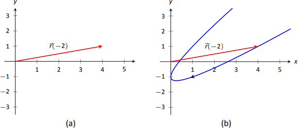
Evaluating a vector-valued function at a specific value of \(t\) is straightforward; simply evaluate each component function at that value of \(t\). For instance, if \(\vecs r(t) = \langle t^2,t^2+t-1\rangle\), then \(\vecs r(-2) = \langle 4,1\rangle\). We can sketch this vector, as is done in Figure \(\PageIndex{1a}\). Plotting lots of vectors is cumbersome, though, so generally we do not sketch the whole vector but just the terminal point. The graph of a vector-valued function is the set of all terminal points of \(\vecs r(t)\), where the initial point of each vector is always the origin. In Figure \(\PageIndex{1b}\) we sketch the graph of \(\vecs r\); we can indicate individual points on the graph with their respective vector, as shown.
Vector-valued functions are closely related to parametric equations of graphs. While in both methods we plot points \(\big(x(t), y(t)\big)\) or \(\big(x(t),y(t),z(t)\big)\) to produce a graph, in the context of vector-valued functions each such point represents a vector. The implications of this will be more fully realized in the next section as we apply calculus ideas to these functions.
Example \(\PageIndex{1}\): Graphing vector-valued functions
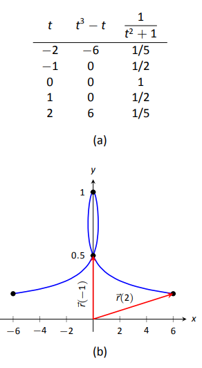
Graph \( \vecs r(t) = \langle t^3-t, \dfrac{1}{t^2+1}\rangle\), for \(-2\leq t\leq 2\). Sketch \(\vecs r(-1)\) and \(\vecs r(2)\).
Solution
We start by making a table of \(t\), \(x\) and \(y\) values as shown in Figure \(\PageIndex{1a}\). Plotting these points gives an indication of what the graph looks like. In Figure \(\PageIndex{1b}\), we indicate these points and sketch the full graph. We also highlight \(\vecs r(-1)\) and \(\vecs r(2)\) on the graph.
Example \(\PageIndex{2}\): Graphing vector-valued functions.
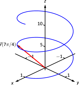
Graph \(\vecs r(t) = \langle \cos t,\sin t,t\rangle\) for \(0\leq t\leq 4\pi\).
Solution
We can again plot points, but careful consideration of this function is very revealing. Momentarily ignoring the third component, we see the \(x\) and \(y\) components trace out a circle of radius 1 centered at the origin. Noticing that the \(z\) component is \(t\), we see that as the graph winds around the \(z\)-axis, it is also increasing at a constant rate in the positive \(z\) direction, forming a spiral. This is graphed in Figure \(\PageIndex{3}\). In the graph \(\vecs r(7\pi/4)\approx (0.707,-0.707,5.498) \) is highlighted to help us understand the graph.
Algebra of Vector-Valued Functions
Definition \(\PageIndex{2}\): Operations on Vector-Valued Functions
Let \(\vecs r_1(t)=\langle f_1(t),g_1(t)\rangle\) and \(\vecs r_2(t)=\langle f_2(t),g_2(t)\rangle\) be vector-valued functions in \(\mathbb{R}^2\) and let \(c\) be a scalar. Then:
- \(\vecs r_1(t) \pm \vecs r_2(t) = \langle\, f_1(t)\pm f_2(t),g_1(t)\pm g_2(t)\,\rangle\).
- \(c\vecs r_1(t) = \langle\, cf_1(t),cg_1(t)\,\rangle\).
A similar definition holds for vector-valued functions in \(\mathbb{R}^3\).
This definition states that we add, subtract and scale vector-valued functions component-wise. Combining vector-valued functions in this way can be very useful (as well as create interesting graphs).
Example \(\PageIndex{3}\): Adding and scaling vector-valued functions.
Let \(\vecs r_1(t) = \langle\,0.2t,0.3t\,\rangle\), \(\vecs r_2(t) = \langle\,\cos t,\sin t\,\rangle\) and \(\vecs r(t) = \vecs r_1(t)+\vecs r_2(t)\). Graph \(\vecs r_1(t)\), \(\vecs r_2(t)\), \(\vecs r(t)\) and \(5\vecs r(t)\) on \(-10\leq t\leq10\).
Solution
We can graph \(\vecs r_1\) and \(\vecs r_2\) easily by plotting points (or just using technology). Let's think about each for a moment to better understand how vector-valued functions work.
We can rewrite \(\vecs r_1(t) = \langle\, 0.2t,0.3t\,\rangle\) as \( \vecs r_1(t) = t\langle 0.2,0.3\rangle\). That is, the function \(\vecs r_1\) scales the vector \(\langle 0.2,0.3\rangle\) by \(t\). This scaling of a vector produces a line in the direction of \(\langle 0.2,0.3\rangle\).
We are familiar with \(\vecs r_2(t) = \langle\, \cos t,\sin t\,\rangle\); it traces out a circle, centered at the origin, of radius 1. Figure \(\PageIndex{4a}\) graphs \(\vecs r_1(t)\) and \(\vecs r_2(t)\).
Adding \(\vecs r_1(t)\) to \(\vecs r_2(t)\) produces \(\vecs r(t) = \langle\,\cos t + 0.2t,\sin t+0.3t\,\rangle\), graphed in Figure \(\PageIndex{4b}\). The linear movement of the line combines with the circle to create loops that move in the direction of \(\langle 0.2,0.3\rangle\). (We encourage the reader to experiment by changing \(\vecs r_1(t)\) to \(\langle 2t,3t\rangle\), etc., and observe the effects on the loops.)
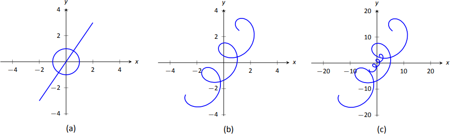
Multiplying \(\vecs r(t)\) by 5 scales the function by 5, producing \(5\vecs r(t) = \langle 5\cos t+1,5\sin t+1.5\rangle\), which is graphed in Figure \(\PageIndex{4c}\) along with \(\vecs r(t)\). The new function is "5 times bigger'' than \(\vecs r(t)\). Note how the graph of \(5\vecs r(t)\) in (c) looks identical to the graph of \(\vecs r(t)\) in \((b)\). This is due to the fact that the \(x\) and \(y\) bounds of the plot in \((c)\) are exactly 5 times larger than the bounds in (b).
Example \(\PageIndex{4}\): Adding and scaling vector-valued functions.
A cycloid is a graph traced by a point \(p\) on a rolling circle, as shown in Figure \(\PageIndex{5}\). Find an equation describing the cycloid, where the circle has radius 1.
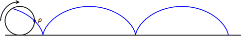
Solution
This problem is not very difficult if we approach it in a clever way. We start by letting \(\vecs p(t)\) describe the position of the point \(p\) on the circle, where the circle is centered at the origin and only rotates clockwise (i.e., it does not roll). This is relatively simple given our previous experiences with parametric equations; \(\vecs p(t) = \langle \cos t, -\sin t\rangle\).
We now want the circle to roll. We represent this by letting \(\vecs c(t)\) represent the location of the center of the circle. It should be clear that the \(y\) component of \(\vecs c(t)\) should be 1; the center of the circle is always going to be 1 if it rolls on a horizontal surface.
The \(x\) component of \(\vecs c(t)\) is a linear function of \(t\): \(f(t) = mt\) for some scalar \(m\). When \(t=0\), \(f(t) = 0\) (the circle starts centered on the \(y\)-axis). When \(t=2\pi\), the circle has made one complete revolution, traveling a distance equal to its circumference, which is also \(2\pi\). This gives us a point on our line \(f(t) = mt\), the point \((2\pi, 2\pi)\). It should be clear that \(m=1\) and \(f(t) = t\). So \(\vecs c(t) = \langle t, 1\rangle\).
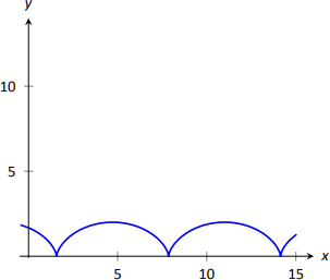
We now combine \(\vecs p\) and \(\vecs c\) together to form the equation of the cycloid:
\[\vecs r(t) = \vecs p(t) + \vecs c(t) = \langle \cos t+ t,-\sin t+1\rangle, \nonumber\]
which is graphed in Figure \(\PageIndex{6}\).
Displacement
A vector-valued function \(\vecs r(t)\) is often used to describe the position of a moving object at time \(t\). At \(t=t_0\), the object is at \(\vecs r(t_0)\); at \(t=t_1\), the object is at \(\vecs r(t_1)\). Knowing the locations \(\vecs r(t_0)\) and \(\vecs r(t_1)\) give no indication of the path taken between them, but often we only care about the difference of the locations, \(\vecs r(t_1)-\vecs r(t_0)\), the displacement.
Definition \(\PageIndex{3}\): Displacement
Let \(\vecs r(t)\) be a vector-valued function and let \(t_0<t_1\) be values in the domain. The displacement \(\vecs d\) of \(\vecs r\), from \(t=t_0\) to \(t=t_1\), is \[\vecs d=\vecs r(t_1)-\vecs r(t_0).\]
When the displacement vector is drawn with initial point at \(\vecs r(t_0)\), its terminal point is \(\vecs r(t_1)\). We think of it as the vector which points from a starting position to an ending position.
Example \(\PageIndex{5}\): Finding and graphing displacement vectors
Let \(\vecs r(t) = \langle \cos (\dfrac{\pi}{2}t),\sin (\dfrac{\pi}2 t)\rangle\). Graph \(\vecs r(t)\) on \(-1\leq t\leq 1\), and find the displacement of \(\vecs r(t)\) on this interval.
Solution
The function \(\vecs r(t)\) traces out the unit circle, though at a different rate than the "usual'' \(\langle \cos t,\sin t\rangle\) parametrization. At \(t_0=-1\), we have \(\vecs r(t_0) = \langle 0,-1\rangle\); at \(t_1=1\), we have \(\vecs r(t_1) = \langle 0,1\rangle\). The displacement of \(\vecs r(t)\) on \([-1,1]\) is thus
\[\vecs d = \langle 0,1\rangle - \langle 0,-1\rangle = \langle 0,2\rangle. \nonumber\]
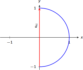
A graph of \(\vecs r(t)\) on \([-1,1]\) is given in Figure \(\PageIndex{7}\), along with the displacement vector \(\vecs d\) on this interval.
Measuring displacement makes us contemplate related, yet very different, concepts. Considering the semi-circular path the object in Example \(\PageIndex{5}\) took, we can quickly verify that the object ended up a distance of 2 units from its initial location. That is, we can compute \(\norm{d} = 2\). However, measuring distance from the starting point is different from measuring distance traveled. Being a semi-circle, we can measure the distance traveled by this object as \(\pi\approx 3.14\) units. Knowing distance from the starting point allows us to compute average rate of change.
Definition \(\PageIndex{4}\): Average Rate of Change
Let \(\vecs r(t)\) be a vector-valued function, where each of its component functions is continuous on its domain, and let \(t_0<t_1\). The average rate of change of \(\vecs r(t)\) on \([t_0,t_1]\) is
\[\text{average rate of change} = \dfrac{\vecs r(t_1) - \vecs r(t_0)}{t_1-t_0}.\]
Example \(\PageIndex{6}\): Average rate of change
Let \(\vecs r(t) = \langle \cos(\dfrac{\pi}2t),\sin(\dfrac{\pi}2t)\rangle\) as in Example 11.1.5. Find the average rate of change of \(\vecs r(t)\) on \([-1,1]\) and on \([-1,5]\).
Solution
We computed in Example \(\PageIndex{5}\) that the displacement of \(\vecs r(t)\) on \([-1,1]\) was \(\vecs d = \langle 0,2\rangle\). Thus the average rate of change of \(\vecs r(t)\) on \([-1,1]\) is:
\[\dfrac{\vecs r(1) -\vecs r(-1)}{1-(-1)} = \dfrac{\langle 0,2\rangle}{2} = \langle 0,1\rangle. \nonumber\]
We interpret this as follows: the object followed a semi-circular path, meaning it moved towards the right then moved back to the left, while climbing slowly, then quickly, then slowly again. On average, however, it progressed straight up at a constant rate of \(\langle 0,1\rangle\) per unit of time.
We can quickly see that the displacement on \([-1,5]\) is the same as on \([-1,1]\), so \(\vecs d = \langle 0,2\rangle\). The average rate of change is different, though:
\[\dfrac{\vecs r(5)-\vecs r(-1)}{5-(-1)} = \dfrac{\langle 0,2\rangle}{6} = \langle 0,1/3\rangle. \nonumber\]
As it took "3 times as long'' to arrive at the same place, this average rate of change on \([-1,5]\) is \(1/3\) the average rate of change on \([-1,1]\).
We considered average rates of change in Sections 1.1 and 2.1 as we studied limits and derivatives. The same is true here; in the following section we apply calculus concepts to vector-valued functions as we find limits, derivatives, and integrals. Understanding the average rate of change will give us an understanding of the derivative; displacement gives us one application of integration.
Contributors and Attributions
Gregory Hartman (Virginia Military Institute). Contributions were made by Troy Siemers and Dimplekumar Chalishajar of VMI and Brian Heinold of Mount Saint Mary's University. This content is copyrighted by a Creative Commons Attribution - Noncommercial (BY-NC) License. http://www.apexcalculus.com/