6.4: Linear Approximations
- Page ID
- 447

\( \newcommand{\vecs}[1]{\overset { \scriptstyle \rightharpoonup} {\mathbf{#1}} } \)
\( \newcommand{\vecd}[1]{\overset{-\!-\!\rightharpoonup}{\vphantom{a}\smash {#1}}} \)
\( \newcommand{\dsum}{\displaystyle\sum\limits} \)
\( \newcommand{\dint}{\displaystyle\int\limits} \)
\( \newcommand{\dlim}{\displaystyle\lim\limits} \)
\( \newcommand{\id}{\mathrm{id}}\) \( \newcommand{\Span}{\mathrm{span}}\)
( \newcommand{\kernel}{\mathrm{null}\,}\) \( \newcommand{\range}{\mathrm{range}\,}\)
\( \newcommand{\RealPart}{\mathrm{Re}}\) \( \newcommand{\ImaginaryPart}{\mathrm{Im}}\)
\( \newcommand{\Argument}{\mathrm{Arg}}\) \( \newcommand{\norm}[1]{\| #1 \|}\)
\( \newcommand{\inner}[2]{\langle #1, #2 \rangle}\)
\( \newcommand{\Span}{\mathrm{span}}\)
\( \newcommand{\id}{\mathrm{id}}\)
\( \newcommand{\Span}{\mathrm{span}}\)
\( \newcommand{\kernel}{\mathrm{null}\,}\)
\( \newcommand{\range}{\mathrm{range}\,}\)
\( \newcommand{\RealPart}{\mathrm{Re}}\)
\( \newcommand{\ImaginaryPart}{\mathrm{Im}}\)
\( \newcommand{\Argument}{\mathrm{Arg}}\)
\( \newcommand{\norm}[1]{\| #1 \|}\)
\( \newcommand{\inner}[2]{\langle #1, #2 \rangle}\)
\( \newcommand{\Span}{\mathrm{span}}\) \( \newcommand{\AA}{\unicode[.8,0]{x212B}}\)
\( \newcommand{\vectorA}[1]{\vec{#1}} % arrow\)
\( \newcommand{\vectorAt}[1]{\vec{\text{#1}}} % arrow\)
\( \newcommand{\vectorB}[1]{\overset { \scriptstyle \rightharpoonup} {\mathbf{#1}} } \)
\( \newcommand{\vectorC}[1]{\textbf{#1}} \)
\( \newcommand{\vectorD}[1]{\overrightarrow{#1}} \)
\( \newcommand{\vectorDt}[1]{\overrightarrow{\text{#1}}} \)
\( \newcommand{\vectE}[1]{\overset{-\!-\!\rightharpoonup}{\vphantom{a}\smash{\mathbf {#1}}}} \)
\( \newcommand{\vecs}[1]{\overset { \scriptstyle \rightharpoonup} {\mathbf{#1}} } \)
\(\newcommand{\longvect}{\overrightarrow}\)
\( \newcommand{\vecd}[1]{\overset{-\!-\!\rightharpoonup}{\vphantom{a}\smash {#1}}} \)
\(\newcommand{\avec}{\mathbf a}\) \(\newcommand{\bvec}{\mathbf b}\) \(\newcommand{\cvec}{\mathbf c}\) \(\newcommand{\dvec}{\mathbf d}\) \(\newcommand{\dtil}{\widetilde{\mathbf d}}\) \(\newcommand{\evec}{\mathbf e}\) \(\newcommand{\fvec}{\mathbf f}\) \(\newcommand{\nvec}{\mathbf n}\) \(\newcommand{\pvec}{\mathbf p}\) \(\newcommand{\qvec}{\mathbf q}\) \(\newcommand{\svec}{\mathbf s}\) \(\newcommand{\tvec}{\mathbf t}\) \(\newcommand{\uvec}{\mathbf u}\) \(\newcommand{\vvec}{\mathbf v}\) \(\newcommand{\wvec}{\mathbf w}\) \(\newcommand{\xvec}{\mathbf x}\) \(\newcommand{\yvec}{\mathbf y}\) \(\newcommand{\zvec}{\mathbf z}\) \(\newcommand{\rvec}{\mathbf r}\) \(\newcommand{\mvec}{\mathbf m}\) \(\newcommand{\zerovec}{\mathbf 0}\) \(\newcommand{\onevec}{\mathbf 1}\) \(\newcommand{\real}{\mathbb R}\) \(\newcommand{\twovec}[2]{\left[\begin{array}{r}#1 \\ #2 \end{array}\right]}\) \(\newcommand{\ctwovec}[2]{\left[\begin{array}{c}#1 \\ #2 \end{array}\right]}\) \(\newcommand{\threevec}[3]{\left[\begin{array}{r}#1 \\ #2 \\ #3 \end{array}\right]}\) \(\newcommand{\cthreevec}[3]{\left[\begin{array}{c}#1 \\ #2 \\ #3 \end{array}\right]}\) \(\newcommand{\fourvec}[4]{\left[\begin{array}{r}#1 \\ #2 \\ #3 \\ #4 \end{array}\right]}\) \(\newcommand{\cfourvec}[4]{\left[\begin{array}{c}#1 \\ #2 \\ #3 \\ #4 \end{array}\right]}\) \(\newcommand{\fivevec}[5]{\left[\begin{array}{r}#1 \\ #2 \\ #3 \\ #4 \\ #5 \\ \end{array}\right]}\) \(\newcommand{\cfivevec}[5]{\left[\begin{array}{c}#1 \\ #2 \\ #3 \\ #4 \\ #5 \\ \end{array}\right]}\) \(\newcommand{\mattwo}[4]{\left[\begin{array}{rr}#1 \amp #2 \\ #3 \amp #4 \\ \end{array}\right]}\) \(\newcommand{\laspan}[1]{\text{Span}\{#1\}}\) \(\newcommand{\bcal}{\cal B}\) \(\newcommand{\ccal}{\cal C}\) \(\newcommand{\scal}{\cal S}\) \(\newcommand{\wcal}{\cal W}\) \(\newcommand{\ecal}{\cal E}\) \(\newcommand{\coords}[2]{\left\{#1\right\}_{#2}}\) \(\newcommand{\gray}[1]{\color{gray}{#1}}\) \(\newcommand{\lgray}[1]{\color{lightgray}{#1}}\) \(\newcommand{\rank}{\operatorname{rank}}\) \(\newcommand{\row}{\text{Row}}\) \(\newcommand{\col}{\text{Col}}\) \(\renewcommand{\row}{\text{Row}}\) \(\newcommand{\nul}{\text{Nul}}\) \(\newcommand{\var}{\text{Var}}\) \(\newcommand{\corr}{\text{corr}}\) \(\newcommand{\len}[1]{\left|#1\right|}\) \(\newcommand{\bbar}{\overline{\bvec}}\) \(\newcommand{\bhat}{\widehat{\bvec}}\) \(\newcommand{\bperp}{\bvec^\perp}\) \(\newcommand{\xhat}{\widehat{\xvec}}\) \(\newcommand{\vhat}{\widehat{\vvec}}\) \(\newcommand{\uhat}{\widehat{\uvec}}\) \(\newcommand{\what}{\widehat{\wvec}}\) \(\newcommand{\Sighat}{\widehat{\Sigma}}\) \(\newcommand{\lt}{<}\) \(\newcommand{\gt}{>}\) \(\newcommand{\amp}{&}\) \(\definecolor{fillinmathshade}{gray}{0.9}\)Newton's method is one example of the usefulness of the tangent line as an approximation to a curve. Here we explore another such application. Recall that the tangent line to \(f(x)\) at a point \(x=a\) is given by \(L(x) = f'(a) (x-a) + f(a)\). The tangent line in this context is also called the linear approximation to \(f\) at \(a\).
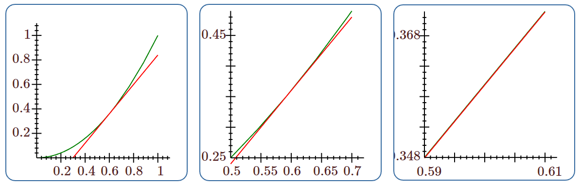
If \(f\) is differentiable at \(a\) then \(L\) is a good approximation of \(f\) so long as \(x\) is "not too far'' from \(a\). Put another way, if \(f\) is differentiable at \(a\) then under a microscope \(f\) will look very much like a straight line. Figure \(\PageIndex{1}\) shows a tangent line to \( y=x^2\) at three different magnifications.
If we want to approximate \(f(b)\), because computing it exactly is difficult, we can approximate the value using a linear approximation, provided that we can compute the tangent line at some \(a\) close to \(b\).
Let \( f(x)=\sqrt{x+4}\). Then \(f'(x)=1/(2\sqrt{x+4})\). The linear approximation to \(f\) at \(x=5\) is
\[L(x)=1/(2\sqrt{5+4})(x-5)+\sqrt{5+4}=(x-5)/6+3. \nonumber \]
As an immediate application we can approximate square roots of numbers near 9 by hand. To estimate \(\sqrt{10}\), we substitute 6 into the linear approximation instead of into \(f(x)\), so
\[ \sqrt{6+4}\approx \dfrac{6-5}{6}+3 = \dfrac{19}{6} \approx 3.1 \overline{6}. \nonumber \]
This rounds to \(3.17\) while the square root of 10 is actually \(3.16\) to two decimal places, so this estimate is only accurate to one decimal place. This is not too surprising, as 10 is really not very close to 9; on the other hand, for many calculations, \(3.2\) would be accurate enough.
With modern calculators and computing software it may not appear necessary to use linear approximations. But in fact they are quite useful. In cases requiring an explicit numerical approximation, they allow us to get a quick rough estimate which can be used as a "reality check'' on a more complex calculation. In some complex calculations involving functions, the linear approximation makes an otherwise intractable calculation possible, without serious loss of accuracy.
Consider the trigonometric function \(\sin x\). Its linear approximation at \(x=0\) is simply \(L(x)=x\). When \(x\) is small this is quite a good approximation and is used frequently by engineers and scientists to simplify some calculations.
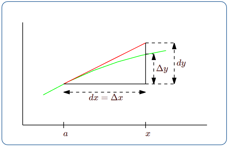
Let \(y=f(x)\) be a differentiable function. We define a new independent variable \(dx\), and a new dependent variable \(dy=f'(x)\,dx\). Notice that \(dy\) is a function both of \(x\) (since \(f'(x)\) is a function of \(x\)) and of \(dx\). We say that \(dx\) and \(dy\) are differentials.
Let \(\Delta x =x-a\) and \(\Delta y= f(x)-f(a)\). If \(x\) is near \(a\) then \(\Delta x\) is small. If we set \(dx=\Delta x\) then
\[dy = f'(a)\,dx \approx {\Delta y\over\Delta x}\Delta x = \Delta y. \nonumber \]
Thus, \(dy\) can be used to approximate \(\Delta y\), the actual change in the function \(f\) between \(a\) and \(x\). This is exactly the approximation given by the tangent line:
\[dy = f'(a)(x-a) = f'(a)(x-a)+f(a)-f(a)=L(x)-f(a). \nonumber \]
While \(L(x)\) approximates \(f(x)\), \(dy\) approximates how \(f(x)\) has changed from \(f(a)\). Figure \(\PageIndex{2}\) illustrates the relationships.