8.4: The Logistic Equation

Learning Objectives

• Describe the concept of environmental carrying capacity in the logistic model of population growth.
• Draw a direction field for a logistic equation and interpret the solution curves.
• Solve a logistic equation and interpret the results.

Differential equations can be used to represent the size of a population as it varies over time. We saw this in an earlier chapter in the section on exponential growth and decay, which is the simplest model. A more realistic model includes other factors that affect the growth of the population. In this section, we study the logistic differential equation and see how it applies to the study of population dynamics in the context of biology.

Population Growth and Carrying Capacity

To model population growth using a differential equation, we first need to introduce some variables and relevant terms. The variable $t$. will represent time. The units of time can be hours, days, weeks, months, or even years. Any given problem must specify the units used in that particular problem. The variable $P$ will represent population. Since the population varies over time, it is understood to be a function of time. Therefore we use the notation $P(t)$ for the population as a function of time. If $P(t)$ is a differentiable function, then the first derivative $\frac{dP}{dt}$ represents the instantaneous rate of change of the population as a function of time.

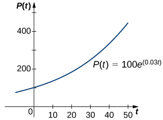
In Exponential Growth and Decay, we studied the exponential growth and decay of populations and radioactive substances. An example of an exponential growth function is $P(t)=P_0e^{rt}.$ In this function, $P(t)$ represents the population at time $t,P_0$ represents the initial population (population at time $t=0$), and the constant $r>0$ is called the growth rate. Figure $\PageIndex{1}$ shows a graph of $P(t)=100e^{0.03t}$. Here $P_0=100$ and $r=0.03$.

Figure $\PageIndex{1}$: An exponential growth model of population.

We can verify that the function $P(t)=P_0e^{rt}$ satisfies the initial-value problem

$$\dfrac{dP}{dt}=rP \nonumber$$

with $P(0)=P_0.$

This differential equation has an interesting interpretation. The left-hand side represents the rate at which the population increases (or decreases). The right-hand side is equal to a positive constant multiplied by the current population. Therefore the differential equation states that the rate at which the population increases is proportional to the population at that point in time. Furthermore, it states that the constant of proportionality never changes.

One problem with this function is its prediction that as time goes on, the population grows without bound. This is unrealistic in a real-world setting. Various factors limit the rate of growth of a particular population, including birth rate, death rate, food supply, predators, and so on. The growth constant $r$ usually takes into consideration the birth and death rates but none of the other factors, and it can be interpreted as a net (birth minus death) percent growth rate per unit time. A natural question to ask is whether the population growth rate stays constant, or whether it changes over time. Biologists have found that in many biological systems, the population grows until a certain steady-state population is reached. This possibility is not taken into account with exponential growth. However, the concept of carrying capacity allows for the possibility that in a given area, only a certain number of a given organism or animal can thrive without running into resource issues.

Definition: Carrying Capacity

The carrying capacity of an organism in a given environment is defined to be the maximum population of that organism that the environment can sustain indefinitely.

We use the variable $K$ to denote the carrying capacity. The growth rate is represented by the variable $r$. Using these variables, we can define the logistic differential equation.

Definition: Logistic Differential Equation

Let $K$ represent the carrying capacity for a particular organism in a given environment, and let $r$ be a real number that represents the growth rate. The function $P(t)$ represents the population of this organism as a function of time $t$, and the constant $P_0$ represents the initial population (population of the organism at time $t=0$). Then the logistic differential equation is

$$\dfrac{dP}{dt}=rP\left(1−\dfrac{P}{K}\right). \label{LogisticDiffEq}$$

The logistic equation was first published by Pierre Verhulst in $1845$. This differential equation can be coupled with the initial condition $P(0)=P_0$ to form an initial-value problem for $P(t).$

Suppose that the initial population is small relative to the carrying capacity. Then $\frac{P}{K}$ is small, possibly close to zero. Thus, the quantity in parentheses on the right-hand side of Equation $\ref{LogisticDiffEq}$ is close to $1$, and the right-hand side of this equation is close to $rP$. If $r>0$, then the population grows rapidly, resembling exponential growth.

However, as the population grows, the ratio $\frac{P}{K}$ also grows, because $K$ is constant. If the population remains below the carrying capacity, then $\frac{P}{K}$ is less than $1$, so $1−\frac{P}{K}>0$. Therefore the right-hand side of Equation $\ref{LogisticDiffEq}$ is still positive, but the quantity in parentheses gets smaller, and the growth rate decreases as a result. If $P=K$ then the right-hand side is equal to zero, and the population does not change.

Now suppose that the population starts at a value higher than the carrying capacity. Then $\frac{P}{K}>1,$ and $1−\frac{P}{K}<0$. Then the right-hand side of Equation $\ref{LogisticDiffEq}$ is negative, and the population decreases. As long as $P>K$, the population decreases. It never actually reaches K because $\frac{dP}{dt}$ will get smaller and smaller, but the population approaches the carrying capacity as $t$ approaches infinity. This analysis can be represented visually by way of a phase line. A phase line describes the general behavior of a solution to an autonomous differential equation, depending on the initial condition. For the case of a carrying capacity in the logistic equation, the phase line is as shown in Figure $\PageIndex{2}$.

Figure $\PageIndex{2}$: A phase line for the differential equation $\dfrac{dP}{dt}=rP(1−\dfrac{P}{K}).$

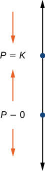
This phase line shows that when $P$ is less than zero or greater than $K$, the population decreases over time. When $P$ is between $0$ and $K$, the population increases over time.

Example $\PageIndex{1}$: Examining the Carrying Capacity of a Deer Population

Let’s consider the population of white-tailed deer (Odocoileus virginianus) in the state of Kentucky. The Kentucky Department of Fish and Wildlife Resources (KDFWR) sets guidelines for hunting and fishing in the state. Before the hunting season of 2004, it estimated a population of 900,000 deer. Johnson notes: “A deer population that has plenty to eat and is not hunted by humans or other predators will double every three years.” (George Johnson, “The Problem of Exploding Deer Populations Has No Attractive Solutions,” January 12,2001, accessed April 9, 2015)

Figure $\PageIndex{3}$: (credit: modification of work by Rachel Kramer, Flickr)

This observation corresponds to a rate of increase $r=\dfrac{\ln (2)}{3}=0.2311,$ so the approximate growth rate is 23.11% per year. (This assumes that the population grows exponentially, which is reasonable––at least in the short term––with plentiful food supply and no predators.) The KDFWR also reports deer population densities for 32 counties in Kentucky, the average of which is approximately 27 deer per square mile. Suppose this is the deer density for the whole state (39,732 square miles). The carrying capacity $K$ is 39,732 square miles times 27 deer per square mile, or 1,072,764 deer.

1. For this application, we have $P_0=900,000,K=1,072,764,$ and $r=0.2311.$ Substitute these values into Equation $\ref{LogisticDiffEq}$ and form the initial-value problem.
2. Solve the initial-value problem from part a.
3. According to this model, what will be the population in $3$ years? Recall that the doubling time predicted by Johnson for the deer population was $3$ years. How do these values compare?

Suppose the population managed to reach 1,200,000 What does the logistic equation predict will happen to the population in this scenario?

Solution

a. The initial value problem is

$$\dfrac{dP}{dt}=0.2311P \left(1−\dfrac{P}{1,072,764}\right),\,\,P(0)=900,000. \nonumber$$

b. The logistic equation is an autonomous differential equation, so we can use the method of separation of variables.

Step 1: Setting the right-hand side equal to zero gives $P=0$ and $P=1,072,764.$ This means that if the population starts at zero it will never change, and if it starts at the carrying capacity, it will never change.

Step 2: Rewrite the differential equation and multiply both sides by:

$$\begin{align*} \dfrac{dP}{dt} =0.2311P\left(\dfrac{1,072,764−P}{1,072,764} \right) \\[4pt] dP =0.2311P\left(\dfrac{1,072,764−P}{1,072,764}\right)dt \\[4pt] \dfrac{dP}{P(1,072,764−P)} =\dfrac{0.2311}{1,072,764}dt. \end{align*}$$

Step 3: Integrate both sides of the equation using partial fraction decomposition:

$$\begin{align*} ∫\dfrac{dP}{P(1,072,764−P)} =∫\dfrac{0.2311}{1,072,764}dt \\[4pt] \dfrac{1}{1,072,764}∫ \left(\dfrac{1}{P}+\dfrac{1}{1,072,764−P}\right)dP =\dfrac{0.2311t}{1,072,764}+C \\[4pt] \dfrac{1}{1,072,764}\left(\ln |P|−\ln |1,072,764−P|\right) =\dfrac{0.2311t}{1,072,764}+C. \end{align*} \nonumber$$

Step 4: Multiply both sides by 1,072,764 and use the quotient rule for logarithms:

$$\ln \left|\dfrac{P}{1,072,764−P}\right|=0.2311t+C_1. \nonumber$$

Here $C_1=1,072,764C.$ Next exponentiate both sides and eliminate the absolute value:

$$\begin{align*} e^{\ln \left|\dfrac{P}{1,072,764−P} \right|} =e^{0.2311t + C_1} \\[4pt] \left|\dfrac{P}{1,072,764 - P}\right| =C_2e^{0.2311t} \\[4pt] \dfrac{P}{1,072,764−P} =C_2e^{0.2311t}. \end{align*}$$

Here $C_2=e^{C_1}$ but after eliminating the absolute value, it can be negative as well. Now solve for:

$$\begin{align*} P =C_2e^{0.2311t}(1,072,764−P) \\[4pt] P =1,072,764C_2e^{0.2311t}−C_2Pe^{0.2311t} \\[4pt] P + C_2Pe^{0.2311t} = 1,072,764C_2e^{0.2311t} \\[4pt] P(1+C_2e^{0.2311t} =1,072,764C_2e^{0.2311t} \\[4pt] P(t) =\dfrac{1,072,764C_2e^{0.2311t}}{1+C_2e^{0.23\nonumber11t}}. \end{align*}$$

Step 5: To determine the value of $C_2$, it is actually easier to go back a couple of steps to where $C_2$ was defined. In particular, use the equation

$$\dfrac{P}{1,072,764−P}=C_2e^{0.2311t}. \nonumber$$

The initial condition is $P(0)=900,000$. Replace $P$ with $900,000$ and $t$ with zero:

$$\begin{align*} \dfrac{P}{1,072,764−P} =C_2e^{0.2311t} \\[4pt] \dfrac{900,000}{1,072,764−900,000} =C_2e^{0.2311(0)} \\[4pt] \dfrac{900,000}{172,764} =C_2 \\[4pt] C_2 =\dfrac{25,000}{4,799} \\[4pt] ≈5.209. \end{align*}$$

Therefore

$$\begin{align*} P(t) =\dfrac{1,072,764 \left(\dfrac{25000}{4799}\right)e^{0.2311t}}{1+\left(\dfrac{25000}{4799}\right)e^{0.2311t}}\\[4pt] =\dfrac{1,072,764(25000)e^{0.2311t}}{4799+25000e^{0.2311t}.} \end{align*}$$

Dividing the numerator and denominator by 25,000 gives

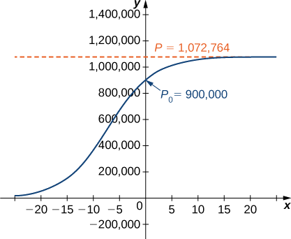
$$P(t)=\dfrac{1,072,764e^{0.2311t}}{0.19196+e^{0.2311t}}. \nonumber$$

Figure $\PageIndex{4}$ is a graph of this equation.

Figure $\PageIndex{4}$: Logistic curve for the deer population with an initial population of 900,000 deer.

c. Using this model we can predict the population in 3 years.

$$P(3)=\dfrac{1,072,764e^{0.2311(3)}}{0.19196+e^{0.2311(3)}}≈978,830\,deer \nonumber$$

This is far short of twice the initial population of $900,000.$ Remember that the doubling time is based on the assumption that the growth rate never changes, but the logistic model takes this possibility into account.

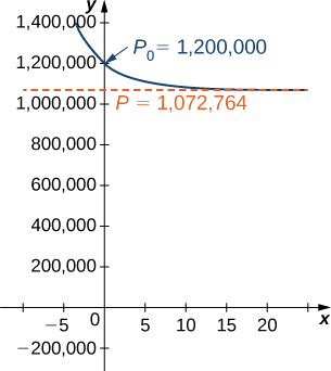
d. If the population reached 1,200,000 deer, then the new initial-value problem would be

$$\dfrac{dP}{dt}=0.2311P \left(1−\dfrac{P}{1,072,764}\right), \, P(0)=1,200,000. \nonumber$$

The general solution to the differential equation would remain the same.

$$P(t)=\dfrac{1,072,764C_2e^{0.2311t}}{1+C_2e^{0.2311t}} \nonumber$$

To determine the value of the constant, return to the equation

$$\dfrac{P}{1,072,764−P}=C_2e^{0.2311t}. \nonumber$$

Substituting the values $t=0$ and $P=1,200,000,$ you get

$$\begin{align*} C_2e^{0.2311(0)} =\dfrac{1,200,000}{1,072,764−1,200,000} \\[4pt] C_2 =−\dfrac{100,000}{10,603}≈−9.431.\end{align*}$$

Therefore

$$\begin{align*} P(t) =\dfrac{1,072,764C_2e^{0.2311t}}{1+C_2e^{0.2311t}} \\[4pt] =\dfrac{1,072,764 \left(−\dfrac{100,000}{10,603}\right)e^{0.2311t}}{1+\left(−\dfrac{100,000}{10,603}\right)e^{0.2311t}} \\[4pt] =−\dfrac{107,276,400,000e^{0.2311t}}{100,000e^{0.2311t}−10,603} \\[4pt] ≈\dfrac{10,117,551e^{0.2311t}}{9.43129e^{0.2311t}−1} \end{align*}$$

This equation is graphed in Figure $\PageIndex{5}$.

Figure $\PageIndex{5}$: Logistic curve for the deer population with an initial population of 1,200,000 deer.

Solving the Logistic Differential Equation

The logistic differential equation is an autonomous differential equation, so we can use separation of variables to find the general solution, as we just did in Example $\PageIndex{1}$.

Step 1: Setting the right-hand side equal to zero leads to $P=0$ and $P=K$ as constant solutions. The first solution indicates that when there are no organisms present, the population will never grow. The second solution indicates that when the population starts at the carrying capacity, it will never change.

Step 2: Rewrite the differential equation in the form

$$\dfrac{dP}{dt}=\dfrac{rP(K−P)}{K}. \nonumber$$

Then multiply both sides by $dt$ and divide both sides by $P(K−P).$ This leads to

$$\dfrac{dP}{P(K−P)}=\dfrac{r}{K}dt. \nonumber$$

Multiply both sides of the equation by $K$ and integrate:

$$∫\dfrac{K}{P(K−P)}dP=∫rdt. \label{eq20a}$$

The left-hand side of this equation can be integrated using partial fraction decomposition. We leave it to you to verify that

$$\dfrac{K}{P(K−P)}=\dfrac{1}{P}+\dfrac{1}{K−P}. \nonumber$$

Then the Equation $\ref{eq20a}$ becomes

$$∫\dfrac{1}{P}+\dfrac{1}{K−P}dP=∫rdt \nonumber$$

$$\ln |P|−\ln |K−P|=rt+C \nonumber$$

$$\ln \left| \dfrac{P}{K−P}\right|=rt+C. \nonumber$$

Now exponentiate both sides of the equation to eliminate the natural logarithm:

$$e^{\ln \left| \tfrac{P}{K−P}\right|}=e^{rt+C} \nonumber$$

$$\left| \dfrac{P}{K−P}\right|=e^Ce^{rt}. \nonumber$$

We define $C_1=e^c$ so that the equation becomes

$$\dfrac{P}{K−P}=C_1e^{rt}. \label{eq30a}$$

To solve this equation for $P(t)$, first multiply both sides by $K−P$ and collect the terms containing $P$ on the left-hand side of the equation:

$$\begin{align*} P =C_1e^{rt}(K−P) \\[4pt] =C_1Ke^{rt}−C_1Pe^{rt} \\[4pt] P+C_1Pe^{rt} =C_1Ke^{rt}.\end{align*}$$

Next, factor $P$ from the left-hand side and divide both sides by the other factor:

$$\begin{align*} P(1+C_1e^{rt}) =C_1Ke^{rt} \\[4pt] P(t) =\dfrac{C_1Ke^{rt}}{1+C_1e^{rt}}. \end{align*}$$

The last step is to determine the value of $C_1.$ The easiest way to do this is to substitute $t=0$ and $P_0$ in place of $P$ in Equation and solve for $C_1$:

$$\begin{align*} \dfrac{P}{K−P} = C_1e^{rt} \\[4pt] \dfrac{P_0}{K−P_0} =C_1e^{r(0)} \\[4pt] C_1 = \dfrac{P_0}{K−P_0}. \end{align*}$$

Finally, substitute the expression for $C_1$ into Equation $\ref{eq30a}$:

$$P(t)=\dfrac{C_1Ke^{rt}}{1+C_1e^{rt}}=\dfrac{\dfrac{P_0}{K−P_0}Ke^{rt}}{1+\dfrac{P_0}{K−P_0}e^{rt}} \nonumber$$

Now multiply the numerator and denominator of the right-hand side by $(K−P_0)$ and simplify:

$$\begin{align*} P(t) &=\dfrac{\dfrac{P_0}{K−P_0}Ke^{rt}}{1+\dfrac{P_0}{K−P_0}e^{rt}} \\[4pt] &=\dfrac{\dfrac{P_0}{K−P_0}Ke^{rt}}{1+\dfrac{P_0}{K−P_0}e^{rt}}⋅\dfrac{K−P_0}{K−P_0} \\[4pt] &=\dfrac{P_0Ke^{rt}}{(K−P_0)+P_0e^{rt}}. \end{align*}$$

We state this result as a theorem.

Solution of the Logistic Differential Equation

Consider the logistic differential equation subject to an initial population of $P_0$ with carrying capacity $K$ and growth rate $r$. The solution to the corresponding initial-value problem is given by

$$P(t)=\dfrac{P_0Ke^{rt}}{(K−P_0)+P_0e^{rt}} \nonumber$$.

Now that we have the solution to the initial-value problem, we can choose values for $P_0,r$, and $K$ and study the solution curve. For example, in Example we used the values $r=0.2311,K=1,072,764,$ and an initial population of $900,000$ deer. This leads to the solution

$$\begin{align*} P(t) =\dfrac{P_0Ke^{rt}}{(K−P_0)+P_0e^{rt}}\\[4pt] =\dfrac{900,000(1,072,764)e^{0.2311t}}{(1,072,764−900,000)+900,000e^{0.2311t}}\\[4pt] =\dfrac{900,000(1,072,764)e^{0.2311t}}{172,764+900,000e^{0.2311t}}.\end{align*}$$

Dividing top and bottom by $900,000$ gives

$$P(t)=\dfrac{1,072,764e^{0.2311t}}{0.19196+e^{0.2311t}}. \nonumber$$

This is the same as the original solution. The graph of this solution is shown again in blue in Figure $\PageIndex{6}$, superimposed over the graph of the exponential growth model with initial population $900,000$ and growth rate $0.2311$ (appearing in green). The red dashed line represents the carrying capacity, and is a horizontal asymptote for the solution to the logistic equation.

Figure $\PageIndex{6}$: A comparison of exponential versus logistic growth for the same initial population of $900,000$ organisms and growth rate of $23.11%.$

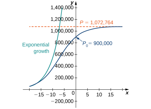
Working under the assumption that the population grows according to the logistic differential equation, this graph predicts that approximately $20$ years earlier $(1984)$, the growth of the population was very close to exponential. The net growth rate at that time would have been around $23.1%$ per year. As time goes on, the two graphs separate. This happens because the population increases, and the logistic differential equation states that the growth rate decreases as the population increases. At the time the population was measured $(2004)$, it was close to carrying capacity, and the population was starting to level off.

The solution to the logistic differential equation has a point of inflection. To find this point, set the second derivative equal to zero:

$$\begin{align*} P(t) =\dfrac{P_0Ke^{rt}}{(K−P_0)+P_0e^{rt}} \\[4pt] P′(t) =\dfrac{rP_0K(K−P_0)e^{rt}}{((K−P_0)+P_0e^{rt})^2} \\[4pt] P''(t) =\dfrac{r^2P_0K(K−P_0)^2e^{rt}−r^2P_0^2K(K−P_0)e^{2rt}}{((K−P_0)+P_0e^{rt})^3} \\[4pt] =\dfrac{r^2P_0K(K−P_0)e^{rt}((K−P_0)−P_0e^{rt})}{((K−P_0)+P_0e^{rt})^3}. \end{align*}$$

Setting the numerator equal to zero,

$$r^2P_0K(K−P_0)e^{rt}((K−P_0)−P_0e^{rt})=0. \nonumber$$

As long as $P_0≠K$, the entire quantity before and including $e^{rt}$is nonzero, so we can divide it out:

$$(K−P_0)−P_0e^{rt}=0. \nonumber$$

Solving for $t$,

$$P_0e^{rt}=K−P_0 \nonumber$$

$$e^{rt}=\dfrac{K−P_0}{P_0} \nonumber$$

$$\ln e^{rt}=\ln \dfrac{K−P_0}{P_0} \nonumber$$

$$rt=\ln \dfrac{K−P_0}{P_0} \nonumber$$

$$t=\dfrac{1}{r}\ln \dfrac{K−P_0}{P_0}. \nonumber$$

Notice that if $P_0>K$, then this quantity is undefined, and the graph does not have a point of inflection. In the logistic graph, the point of inflection can be seen as the point where the graph changes from concave up to concave down. This is where the “leveling off” starts to occur, because the net growth rate becomes slower as the population starts to approach the carrying capacity.

Exercise $\PageIndex{1}$

A population of rabbits in a meadow is observed to be $200$ rabbits at time $t=0$. After a month, the rabbit population is observed to have increased by $4%$. Using an initial population of $200$ and a growth rate of $0.04$, with a carrying capacity of $750$ rabbits,

1. Write the logistic differential equation and initial condition for this model.
2. Draw a slope field for this logistic differential equation, and sketch the solution corresponding to an initial population of $200$ rabbits.
3. Solve the initial-value problem for $P(t)$.
4. Use the solution to predict the population after $1$ year.

Hint

First determine the values of $r,K,$ and $P_0$. Then create the initial-value problem, draw the direction field, and solve the problem.

Answer

a. $\dfrac{dP}{dt}=0.04(1−\dfrac{P}{750}),P(0)=200$

b.

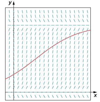
c. $P(t)=\dfrac{3000e^{.04t}}{11+4e^{.04t}}$

d. After $12$ months, the population will be $P(12)≈278$ rabbits.

Student Project: Logistic Equation with a Threshold Population

An improvement to the logistic model includes a threshold population. The threshold population is defined to be the minimum population that is necessary for the species to survive. We use the variable $T$ to represent the threshold population. A differential equation that incorporates both the threshold population $T$ and carrying capacity $K$ is

$$\dfrac{dP}{dt}=−rP\left(1−\dfrac{P}{K}\right)\left(1−\dfrac{P}{T}\right) \nonumber$$

where $r$ represents the growth rate, as before.

1. The threshold population is useful to biologists and can be utilized to determine whether a given species should be placed on the endangered list. A group of Australian researchers say they have determined the threshold population for any species to survive: $5000$ adults. (Catherine Clabby, “A Magic Number,” American Scientist 98(1): 24, doi:10.1511/2010.82.24. accessed April 9, 2015, www.americanscientist.org/iss...a-magic-number). Therefore we use $T=5000$ as the threshold population in this project. Suppose that the environmental carrying capacity in Montana for elk is $25,000$. Set up Equation using the carrying capacity of $25,000$ and threshold population of $5000$. Assume an annual net growth rate of 18%.
2. Draw the direction field for the differential equation from step $1$, along with several solutions for different initial populations. What are the constant solutions of the differential equation? What do these solutions correspond to in the original population model (i.e., in a biological context)?
3. What is the limiting population for each initial population you chose in step $2$? (Hint: use the slope field to see what happens for various initial populations, i.e., look for the horizontal asymptotes of your solutions.)
4. This equation can be solved using the method of separation of variables. However, it is very difficult to get the solution as an explicit function of $t$. Using an initial population of $18,000$ elk, solve the initial-value problem and express the solution as an implicit function of t, or solve the general initial-value problem, finding a solution in terms of $r,K,T,$ and $P_0$.

Key Concepts

• When studying population functions, different assumptions—such as exponential growth, logistic growth, or threshold population—lead to different rates of growth.
• The logistic differential equation incorporates the concept of a carrying capacity. This value is a limiting value on the population for any given environment.
• The logistic differential equation can be solved for any positive growth rate, initial population, and carrying capacity.

Key Equations

• Logistic differential equation and initial-value problem

$\dfrac{dP}{dt}=rP\left(1−\dfrac{P}{K}\right),\quad P(0)=P_0$

• Solution to the logistic differential equation/initial-value problem

$P(t)=\dfrac{P_0Ke^{rt}}{(K−P_0)+P_0e^{rt}}$

• Threshold population model

$\dfrac{dP}{dt}=−rP\left(1−\dfrac{P}{K}\right)\left(1−\dfrac{P}{T}\right)$

Glossary

carrying capacity

the maximum population of an organism that the environment can sustain indefinitely

growth rate

the constant $r>0$ in the exponential growth function $P(t)=P_0e^{rt}$

initial population

the population at time $t=0$

logistic differential equation

a differential equation that incorporates the carrying capacity $K$ and growth rate rr into a population model

phase line

a visual representation of the behavior of solutions to an autonomous differential equation subject to various initial conditions

threshold population

the minimum population that is necessary for a species to survive