1.2: Epsilon-Delta Definition of a Limit

This section introduces the formal definition of a limit. Many refer to this as "the epsilon--delta,'' definition, referring to the letters $\epsilon$ and $\delta$ of the Greek alphabet.

Before we give the actual definition, let's consider a few informal ways of describing a limit. Given a function $y=f(x)$ and an $x$-value, $c$, we say that "the limit of the function $f$, as $x$ approaches $c$, is a value $L$'':

1. if "$y$ tends to $L$'' as "$x$ tends to $c$.''
2. if "$y$ approaches $L$'' as "$x$ approaches $c$.''
3. if "$y$ is near $L$'' whenever "$x$ is near $c$.''

The problem with these definitions is that the words "tends,'' "approach,'' and especially "near'' are not exact. In what way does the variable $x$ tend to, or approach, $c$? How near do $x$ and $y$ have to be to $c$ and $L$, respectively?

The definition we describe in this section comes from formalizing 3. A quick restatement gets us closer to what we want:

$\textbf{3}^\prime$. If $x$ is within a certain tolerance level of $c$, then the corresponding value $y=f(x)$ is within a certain tolerance level of $L$.

The traditional notation for the $x$-tolerance is the lowercase Greek letter delta, or $\delta$, and the $y$-tolerance is denoted by lowercase epsilon, or $\epsilon$. One more rephrasing of $\textbf{3}^\prime$ nearly gets us to the actual definition:

$\textbf{3}^{\prime \prime}$. If $x$ is within $\delta$ units of $c$, then the corresponding value of $y$ is within $\epsilon$ units of $L$.

We can write "$x$ is within $\delta$ units of $c$'' mathematically as

$$|x-c| < \delta, \qquad \text{which is equivalent to }\qquad c-\delta < x < c+\delta.$$

Letting the symbol "$\longrightarrow$'' represent the word "implies,'' we can rewrite $\textbf{3}''$ as

$$|x - c| < \delta \longrightarrow |y - L| < \epsilon \qquad \textrm{or} \qquad c - \delta < x < c + \delta \longrightarrow L - \epsilon < y < L + \epsilon.$$

The point is that $\delta$ and $\epsilon$, being tolerances, can be any positive (but typically small) values. Finally, we have the formal definition of the limit with the notation seen in the previous section.

Definition 1: The Limit of a Function $f$

Let $I$ be an open interval containing $c$, and let $f$ be a function defined on $I$, except possibly at $c$. The limit of $f(x)$, as $x$ approaches $c$, is $L$, denoted by

$$\lim_{x\rightarrow c} f(x) = L,$$

means that given any $\epsilon > 0$, there exists $\delta > 0$ such that for all $x\neq c$, if $|x - c| < \delta$, then $|f(x) - L| < \epsilon$.

(Mathematicians often enjoy writing ideas without using any words. Here is the wordless definition of the limit:

$$\lim_{x\rightarrow c} f(x) = L \iff \forall \, \epsilon > 0, \exists \, \delta > 0 \; s.t. \;0<|x - c| < \delta \longrightarrow |f(x) - L| < \epsilon .\text{)}$$

Note the order in which $\epsilon$ and $\delta$ are given. In the definition, the $y$-tolerance $\epsilon$ is given first and then the limit will exist if we can find an $x$-tolerance $\delta$ that works.

An example will help us understand this definition. Note that the explanation is long, but it will take one through all steps necessary to understand the ideas.

Example 6: Evaluating a limit using the definition

Show that $\lim\limits_{x\rightarrow 4} \sqrt{x} = 2 .$

Solution:
Before we use the formal definition, let's try some numerical tolerances. What if the $y$ tolerance is 0.5, or $\epsilon =0.5$? How close to 4 does $x$ have to be so that $y$ is within 0.5 units of 2, i.e., $1.5 < y < 2.5$? In this case, we can proceed as follows:

$$\begin{align}1.5 &< y < 2.5 \\ 1.5 &< \sqrt{x} < 2.5\\ 1.5^2 &< x < 2.5^2\\ 2.25 &< x < 6.25.\\ \end{align}$$

So, what is the desired $x$ tolerance? Remember, we want to find a symmetric interval of $x$ values, namely $4 - \delta < x < 4 + \delta$. The lower bound of $2.25$ is $1.75$ units from 4; the upper bound of 6.25 is 2.25 units from 4. We need the smaller of these two distances; we must have $\delta \leq 1.75$. See Figure 1.17.

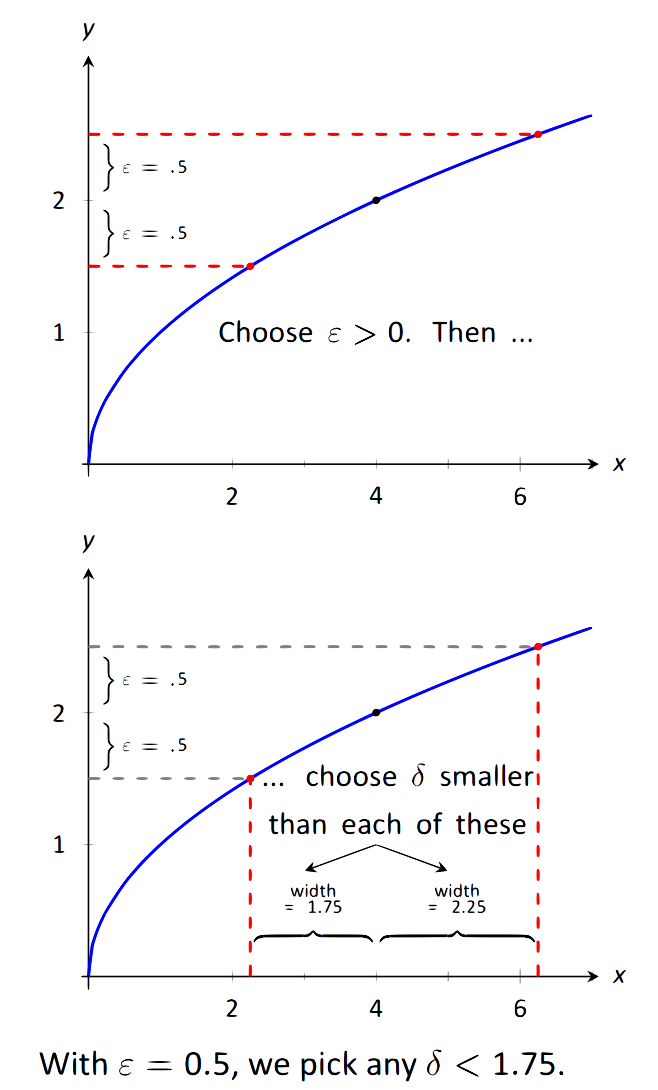
$\text{FIGURE 1.17}$: Illustrating the $\epsilon - \delta$ process.

Given the $y$ tolerance $\epsilon =0.5$, we have found an $x$ tolerance, $\delta \leq 1.75$, such that whenever $x$ is within $\delta$ units of 4, then $y$ is within $\epsilon$ units of 2. That's what we were trying to find.

Let's try another value of $\epsilon$.

What if the $y$ tolerance is 0.01, i.e., $\epsilon =0.01$? How close to 4 does $x$ have to be in order for $y$ to be within 0.01 units of 2 (or $1.99 < y < 2.01$)? Again, we just square these values to get $1.99^2 < x < 2.01^2$, or

$$3.9601 < x < 4.0401.$$

What is the desired $x$ tolerance? In this case we must have $\delta \leq 0.0399$, which is the minimum distance from 4 of the two bounds given above.

Note that in some sense, it looks like there are two tolerances (below 4 of 0.0399 units and above 4 of 0.0401 units). However, we couldn't use the larger value of $0.0401$ for $\delta$ since then the interval for $x$ would be $3.9599 < x < 4.0401$ resulting in $y$ values of $1.98995 < y < 2.01$ (which contains values NOT within 0.01 units of 2).

What we have so far: if $\epsilon =0.5$, then $\delta \leq 1.75$ and if $\epsilon = 0.01$, then $\delta \leq 0.0399$. A pattern is not easy to see, so we switch to general $\epsilon$ try to determine $\delta$ symbolically. We start by assuming $y=\sqrt{x}$ is within $\epsilon$ units of 2:

$$\begin{eqnarray*}|y - 2| < \epsilon &\\ -\epsilon < y - 2 < \epsilon& \qquad \textrm{(Definition of absolute value)}\\ -\epsilon < \sqrt{x} - 2 < \epsilon &\qquad (y=\sqrt{x})\\ 2 - \epsilon < \sqrt{x} < 2+ \epsilon &\qquad \textrm{ (Add 2)}\\ (2 - \epsilon)^2 < x < (2+ \epsilon) ^2 &\qquad \textrm{ (Square all)}\\ 4 - 4\epsilon + \epsilon^2 < x < 4 + 4\epsilon + \epsilon^2 &\qquad \textrm{ (Expand)}\\ 4 - (4\epsilon - \epsilon^2) < x < 4 + (4\epsilon + \epsilon^2). &\qquad \textrm{ (Rewrite in the desired form)}\end{eqnarray*}$$

The "desired form'' in the last step is " $4-\textit{something} < x < 4 +\textit{something}$.'' Since we want this last interval to describe an $x$ tolerance around 4, we have that either $\delta \leq 4\epsilon - \epsilon^2$ or $\delta \leq 4\epsilon + \epsilon^2$, whichever is smaller:

$$\delta \leq \min\{4\epsilon - \epsilon^2, 4\epsilon + \epsilon^2\}.$$

Since $\epsilon > 0$, the minimum is $\delta \leq 4\epsilon - \epsilon^2$. That's the formula: given an $\epsilon$, set $\delta \leq 4\epsilon-\epsilon^2$.

We can check this for our previous values. If $\epsilon=0.5$, the formula gives $\delta \leq 4(0.5) - (0.5)^2 = 1.75$ and when $\epsilon=0.01$, the formula gives $\delta \leq 4(0.01) - (0.01)^2 = 0.399$.

So given any $\epsilon >0$, set $\delta \leq 4\epsilon - \epsilon^2$. Then if $|x-4|<\delta$ (and $x\neq 4$), then $|f(x) - 2| < \epsilon$, satisfying the definition of the limit. We have shown formally (and finally!) that $\lim_{x\rightarrow 4} \sqrt{x} = 2$.

Actually, it is a pain, but this won't work if $\epsilon \ge 4$. This shouldn't really occur since $\epsilon$ is supposed to be small, but it could happen. In the cases where $\epsilon \ge 4$, just take $\delta = 1$ and you'll be fine.

The previous example was a little long in that we sampled a few specific cases of $\epsilon$ before handling the general case. Normally this is not done. The previous example is also a bit unsatisfying in that $\sqrt{4}=2$; why work so hard to prove something so obvious? Many $\epsilon$-$\delta$ proofs are long and difficult to do. In this section, we will focus on examples where the answer is, frankly, obvious, because the non--obvious examples are even harder. In the next section we will learn some theorems that allow us to evaluate limits analytically, that is, without using the $\epsilon$-$\delta$ definition.

That is why theorems about limits are so useful! After doing a few more $\epsilon$-$\delta$ proofs, you will really appreciate the analytical "short cuts'' found in the next section.

Example 7: Evaluating a limit using the definition

Show that $\lim_{x\rightarrow 2} x^2 = 4$.

Solution

Let's do this example symbolically from the start. Let $\epsilon > 0$ be given; we want $|y-4| < \epsilon$, i.e., $|x^2-4| < \epsilon$. How do we find $\delta$ such that when $|x-2| < \delta$, we are guaranteed that $|x^2-4|<\epsilon$?

This is a bit trickier than the previous example, but let's start by noticing that $|x^2-4| = |x-2|\cdot|x+2|$. Consider:

$$|x^2-4| < \epsilon \longrightarrow |x-2|\cdot|x+2| < \epsilon \longrightarrow |x-2| < \frac{\epsilon}{|x+2|}.\label{eq:limit1}\tag{1.1}$$

Could we not set $\delta = \frac{\epsilon}{|x+2|}$?

We are close to an answer, but the catch is that $\delta$ must be a constant value (so it can't contain $x$). There is a way to work around this, but we do have to make an assumption. Remember that $\epsilon$ is supposed to be a small number, which implies that $\delta$ will also be a small value. In particular, we can (probably) assume that $\delta < 1$. If this is true, then $|x-2| < \delta$ would imply that $|x-2| < 1$, giving $1 < x < 3$.

Now, back to the fraction $\frac{\epsilon}{|x+2|}$. If $1<x<3$, then $3<x+2<5$ (add 2 to all terms in the inequality). Taking reciprocals, we have

$$\begin{align}\frac{1}{5} <& \frac{1}{|x+2|} < \frac {1}{3} & \text{which implies}\\ \frac{1}{5} <& \frac{1}{|x+2|} & \text{which implies}\\ \frac{\epsilon}{5}<&\frac{\epsilon}{|x+2|}.\label{eq:limit2}\tag{1.2}\end{align}$$

This suggests that we set $\delta \leq \frac{\epsilon}{5}$. To see why, let consider what follows when we assume $|x-2|<\delta$:

$$\begin{align*}|x - 2| &< \delta &\\ |x - 2| &< \frac{\epsilon}{5}& \text{(Our choice of \(\delta\))}\\ |x - 2|\cdot|x + 2| &< |x + 2|\cdot\frac{\epsilon}{5}& \text{(Multiply by \(|x+2|\))}\\ |x^2 - 4|&< |x + 2|\cdot\frac{\epsilon}{5}& \text{(Combine left side)}\\ |x^2 - 4|&< |x + 2|\cdot\frac{\epsilon}{5}< |x + 2|\cdot\frac{\epsilon}{|x+2|}=\epsilon & \text{(Using (\ref{eq:limit2}) as long as \(\delta <1\))} \end{align*}$$

We have arrived at $|x^2 - 4|<\epsilon$ as desired. Note again, in order to make this happen we needed $\delta$ to first be less than 1. That is a safe assumption; we want $\epsilon$ to be arbitrarily small, forcing $\delta$ to also be small.

We have also picked $\delta$ to be smaller than "necessary.'' We could get by with a slightly larger $\delta$, as shown in Figure 1.18. The dashed outer lines show the boundaries defined by our choice of $\epsilon$. The dotted inner lines show the boundaries defined by setting $\delta = \epsilon/5$. Note how these dotted lines are within the dashed lines. That is perfectly fine; by choosing $x$ within the dotted lines we are guaranteed that $f(x)$ will be within $\epsilon$ of 4.%If the value we eventually used for $\delta$, namely $\epsilon/5$, is not less than 1, this proof won't work. For the final fix, we instead set $\delta$ to be the minimum of 1 and $\epsilon/5$. This way all calculations above work.

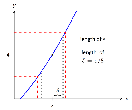
$\text{FIGURE 1.18}$: Choosing $\delta = \epsilon / 5$ in Example 7.

In summary, given $\epsilon > 0$, set $\delta=\leq\epsilon/5$. Then $|x - 2| < \delta$ implies $|x^2 - 4|< \epsilon$ (i.e. $|y - 4|< \epsilon$) as desired. This shows that $\lim_{x\rightarrow 2} x^2 = 4$. Figure 1.18 gives a visualization of this; by restricting $x$ to values within $\delta = \epsilon/5$ of 2, we see that $f(x)$ is within $\epsilon$ of $4$.

Make note of the general pattern exhibited in these last two examples. In some sense, each starts out "backwards.'' That is, while we want to

1. start with $|x-c|<\delta$ and conclude that
2. $|f(x)-L|<\epsilon$,

we actually start by assuming

1. $|f(x)-L|<\epsilon$, then perform some algebraic manipulations to give an inequality of the form
2. $|x-c|<$ something.

When we have properly done this, the something on the "greater than'' side of the inequality becomes our $\delta$. We can refer to this as the "scratch--work'' phase of our proof. Once we have $\delta$, we can formally start with $|x-c|<\delta$ and use algebraic manipulations to conclude that $|f(x)-L|<\epsilon$, usually by using the same steps of our "scratch--work'' in reverse order.

We highlight this process in the following example.

Example 8: Evaluating a limit using the definition

Prove that $\lim\limits_{x\rightarrow 1}x^3-2x = -1$.

Solution

We start our scratch--work by considering $|f(x) - (-1)| < \epsilon$:

$$\begin{align} |f(x)-(-1)| &< \epsilon \\ |x^3-2x + 1|&< \epsilon & \text{(Now factor)}\\ |(x-1)(x^2+x-1)|&< \epsilon \\ |x-1| &<\frac{\epsilon}{|x^2+x-1|}.\label{eq:lim4}\tag{1.3} \end{align}$$

We are at the phase of saying that $|x-1|<$ something, where $\textit{something}=\epsilon/|x^2+x-1|$. We want to turn that something into $\delta$.

Since $x$ is approaching 1, we are safe to assume that $x$ is between 0 and 2. So

$$\begin{align*} 0&< x<2 & \\ 0&< x^2<4.&\text{(squared each term)}\\ \end{align*}$$

Since $0<x<2$, we can add $0$, $x$ and $2$, respectively, to each part of the inequality and maintain the inequality.

$$\begin{align*}0&< x^2+x<6 &\\ -1&< x^2+x-1<5.&\text{(subtracted 1 from each part)} \end{align*}$$

In Equation $\eqref{eq:lim4}$, we wanted $|x-1|<\epsilon/|x^2+x-1|$. The above shows that given any $x$ in $[0,2]$, we know that

$$\begin{align} x^2+x-1 &< 5 &\text{which implies that}\notag\\ \frac15 &< \frac{1}{x^2+x-1} &\text{which implies that}\notag\\ \frac{\epsilon}5 &< \frac{\epsilon}{x^2+x-1}.\label{eq:lim4b}\tag{1.4} \end{align}$$

So we set $\delta \leq \epsilon/5$. This ends our scratch--work, and we begin the formal proof (which also helps us understand why this was a good choice of $\delta$).

Given $\epsilon$, let $\delta \leq \epsilon/5$. We want to show that when $|x-1|<\delta$, then $|(x^3-2x)-(-1)|<\epsilon$. We start with $|x-1|<\delta$:

$$\begin{align*} |x-1| &< \delta \\ |x-1| &< \frac{\epsilon}5\\ |x-1| &< \frac\epsilon5 < \frac{\epsilon}{|x^2+x-1|} & \text{(for \(x\) near 1, from Equation \eqref{eq:lim4b})}\\ |x-1|\cdot |x^2+x-1| &< \epsilon\\ |x^3-2x+1| &< \epsilon\\ |(x^3-2x)-(-1)| &<\epsilon, \end{align*}$$

which is what we wanted to show. Thus $\lim\limits_{x\to 1}x^3-2x = -1$.

We illustrate evaluating limits once more.

Example 9: Evaluating a limit using the definition

Prove that $\lim\limits_{x\rightarrow 0} e^x = 1.$

Solution

Symbolically, we want to take the equation $|e^x - 1| < \epsilon$ and unravel it to the form $|x-0| < \delta$. Here is our scratch--work:

$$\begin{eqnarray*}|e^x - 1| < \epsilon&\\ -\epsilon < e^x - 1 < \epsilon& \qquad \textrm{(Definition of absolute value)}\\ 1-\epsilon < e^x < 1+\epsilon & \qquad \textrm{(Add 1)}\\ \ln(1-\epsilon) < x < \ln(1+\epsilon) & \qquad \textrm{(Take natural logs)}\\ \end{eqnarray*}$$

Making the safe assumption that $\epsilon<1$ ensures the last inequality is valid (i.e., so that $\ln (1-\epsilon)$ is defined). We can then set $\delta$ to be the minimum of $|\ln(1-\epsilon)|$ and $\ln(1+\epsilon)$; i.e.,

$$\delta = \min\{|\ln(1-\epsilon)|, \ln(1+\epsilon)\} = \ln(1+\epsilon).$$

Recall $\ln 1= 0$ and $\ln x<0$ when $0<x<1$. So $\ln (1-\epsilon) <0$, hence we consider its absolute value.

Now, we work through the actual the proof:

$$\begin{align*} |x - 0|&<\delta\\ -\delta &< x < \delta & \textrm{(Definition of absolute value)}\\ -\ln(1+\epsilon) &< x < \ln(1+\epsilon). &\\ \ln(1-\epsilon) &< x < \ln(1+\epsilon). & \text{(since \(\ln(1-\epsilon) < -\ln(1+\epsilon)\))}\\ \end{align*}$$

The above line is true by our choice of $\delta$ and by the fact that since $|\ln(1-\epsilon)|>\ln(1+\epsilon)$ and $\ln(1-\epsilon)<0$, we know $\ln(1-\epsilon) < -\ln(1+\epsilon )$.

$$\begin{align*}1-\epsilon &< e^x < 1+\epsilon & \textrm{(Exponentiate)}\\ -\epsilon &< e^x - 1 < \epsilon & \textrm{(Subtract 1)}\\ \end{align*}$$

In summary, given $\epsilon > 0$, let $\delta = \ln(1+\epsilon)$. Then $|x - 0| < \delta$ implies $|e^x - 1|< \epsilon$ as desired. We have shown that $\displaystyle \lim_{x\rightarrow 0} e^x = 1 .$

We note that we could actually show that $\lim_{x\rightarrow c} e^x = e^c$ for any constant $c$. We do this by factoring out $e^c$ from both sides, leaving us to show $\lim_{x\rightarrow c} e^{x-c} = 1$ instead. By using the substitution $u=x-c$, this reduces to showing $\lim_{u\rightarrow 0} e^u = 1$ which we just did in the last example. As an added benefit, this shows that in fact the function $f(x)=e^x$ is continuous at all values of $x$, an important concept we will define in Section 1.5.

This formal definition of the limit is not an easy concept grasp. Our examples are actually "easy'' examples, using "simple'' functions like polynomials, square--roots and exponentials. It is very difficult to prove, using the techniques given above, that $\lim\limits_{x\to 0}(\sin x)/x = 1$, as we approximated in the previous section.

There is hope. The next section shows how one can evaluate complicated limits using certain basic limits as building blocks. While limits are an incredibly important part of calculus (and hence much of higher mathematics), rarely are limits evaluated using the definition. Rather, the techniques of the following section are employed.

Contributors and Attributions

• Gregory Hartman (Virginia Military Institute). Contributions were made by Troy Siemers and Dimplekumar Chalishajar of VMI and Brian Heinold of Mount Saint Mary's University. This content is copyrighted by a Creative Commons Attribution - Noncommercial (BY-NC) License. http://www.apexcalculus.com/