7.1: Area Between Curves

We begin this chapter with a reminder of a few key concepts from Chapter 5. Let \(f\) be a continuous function on \([a,b]\) which is partitioned into \(n\) subintervals as

$$a<x_1 < x_2 < \cdots < x_n<x_{n+1}=b.\]

Let \(dx_i\) denote the length of the \(i^\text{ th}\) subinterval, and let \(c_i\) be any \(x\)-value in that subinterval. Definition 5.3.1 states that the sum

$$\sum_{i=1}^n f(c_i)\ dx_i\]

is a Riemann Sum. Riemann Sums are often used to approximate some quantity (area, volume, work, pressure, etc.). The approximation becomes exact by taking the limit

$$\lim_{||dx_i||\to0} \sum_{i=1}^n f(c_i) \ dx_i,\]

where \(||\ dx_i||\) the length of the largest subinterval in the partition. Theorem 5.3.2 connects limits of Riemann Sums to definite integrals:

$$\lim_{||dx_i||\to0} \sum_{i=1}^n f(c_i)\ dx_i = \int_a^b f(x)\ dx.\]

Finally, the Fundamental Theorem of Calculus states how definite integrals can be evaluated using antiderivatives.

This chapter employs the following technique to a variety of applications. Suppose the value \(Q\) of a quantity is to be calculated. We first approximate the value of \(Q\) using a Riemann Sum, then find the exact value via a definite integral. We spell out this technique in the following Key Idea.

Key Idea 22: Definite Integral Strategy

Let a quantity be given whose value \(Q\) is to be computed.

1. Divide the quantity into \(n\) smaller "subquantities" of value \(Q_i\).
2. Identify a variable \(x\) and function \(f(x)\) such that each subquantity can be approximated with the product \(f(c_i)\ dx_i\), where \(dx_i\) represents a small change in \(x\). Thus \(Q_i \approx f(c_i)\ dx_i\). A sample approximation \(f(c_i)\ dx_i\) of \(Q_i\) is called a differential element.
3. Recognize that \( Q= \sum_{i=1}^n Q_i \approx \sum_{i=1}^n f(c_i)\ dx_i\), which is a Riemann Sum.
4. Taking the appropriate limit gives \( Q = \int_a^b f(x)\ dx\)

This Key Idea will make more sense after we have had a chance to use it several times. We begin with Area Between Curves, which we addressed briefly in Section 5.5.4.

Area Between Curves

We are often interested in knowing the area of a region. Forget momentarily that we addressed this already in Section 5.5.4 and approach it instead using the technique described in Key Idea 22.

Let \(Q\) be the area of a region bounded by continuous functions \(f\) and \(g\). If we break the region into many subregions, we have an obvious equation:

\[\text{Total Area} = \text{sum of the areas of the subregions.}\]

The issue to address next is how to systematically break a region into subregions. A graph will help. Consider Figure \(\PageIndex{1a}\) where a region between two curves is shaded. While there are many ways to break this into subregions, one particularly efficient way is to "slice" it vertically, as shown in Figure \(\PageIndex{1b}\), into \(n\) equally spaced slices.

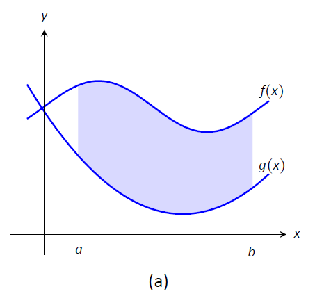
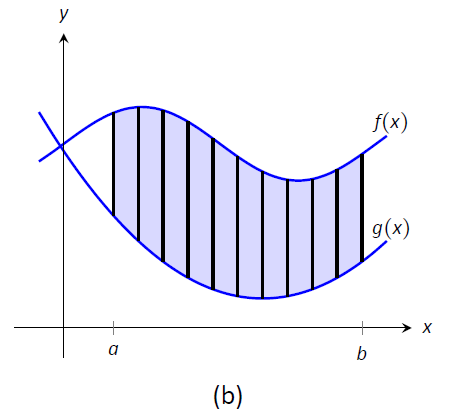
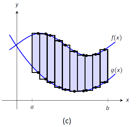
Figure \(\PageIndex{1}\): Subdividing a region into vertical slices and approximating the areas with rectangles.

We now approximate the area of a slice. Again, we have many options, but using a rectangle seems simplest. Picking any \(x\)-value \(c_i\) in the \(i^\text{ th}\) slice, we set the height of the rectangle to be \(f(c_i)-g(c_i)\), the difference of the corresponding \(y\)-values. The width of the rectangle is a small difference in \(x\)-values, which we represent with \(dx\). Figure \(\PageIndex{1c}\) shows sample points \(c_i\) chosen in each subinterval and appropriate rectangles drawn. (Each of these rectangles represents a differential element.) Each slice has an area approximately equal to \(\big(f(c_i)-g(c_i)\big)\ dx\); hence, the total area is approximately the Riemann Sum

$$Q = \sum_{i=1}^n \big(f(c_i)-g(c_i)\big)\ dx.\]

Taking the limit as \(n\to \infty\) gives the exact area as \(\int_a^b \big(f(x)-g(x)\big)\ dx.\)

Theroem \(\PageIndex{1}\): Area Between Curves

Let \(f(x)\) and \(g(x)\) be continuous functions defined on \([a,b]\) where \(f(x)\geq g(x)\) for all \(x\) in \([a,b]\). The area of the region bounded by the curves \(y=f(x)\), \(y=g(x)\) and the lines \(x=a\) and \(x=b\) is

$$\int_a^b \big(f(x)-g(x)\big)\ dx.\]

Example \(\PageIndex{1}\): Finding area enclosed by curves

Find the area of the region bounded by \(f(x) = \sin x+2\), \(g(x) = \dfrac12\cos (2x)-1\), \(x=0\) and \(x=4\pi\), as shown in Figure \(\PageIndex{2}\).

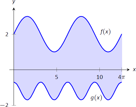
Figure \(\PageIndex{2}\): Graphing an enclosed region in Example \(\PageIndex{1}\).

Solution

The graph verifies that the upper boundary of the region is given by \(f\) and the lower bound is given by \(g\). Therefore the area of the region is the value of the integral

\[\begin{align*}\int_0^{4\pi} \big(f(x)- g(x)\big)\ dx & = \int_0^{4\pi} \Big(\sin x+2 - \big(\dfrac12\cos (2x)-1\big)\Big)\ dx \\[4pt]&= -\cos x -\dfrac14\sin(2x)+3x\Big|_0^{4\pi}\\[4pt] &= 12\pi \approx 37.7\ \text{units}^2.\end{align*}\]

Example \(\PageIndex{2}\): Finding total area enclosed by curves

Find the total area of the region enclosed by the functions \(f(x) = -2x+5\) and \(g(x) = x^3-7x^2+12x-3\) as shown in Figure \(\PageIndex{3}\).

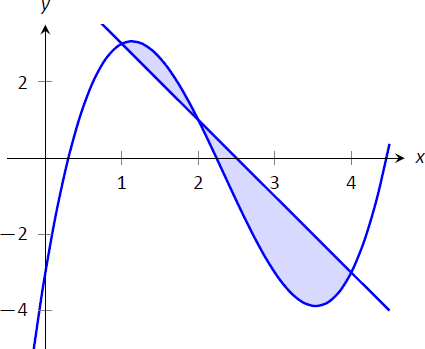
FIgure \(\PageIndex{3}\): Graphing a region enclosed by two functions in Example \(\PageIndex{2}\).

Solution

A quick calculation shows that \(f=g\) at \(x=1, 2\) and 4. One can proceed thoughtlessly by computing \( \int_1^4\big(f(x)-g(x)\big)\ dx\), but this ignores the fact that on \([1,2]\), \(g(x)>f(x)\). (In fact, the thoughtless integration returns \(-9/4\), hardly the expected value of an area.) Thus we compute the total area by breaking the interval \([1,4]\) into two subintervals, \([1,2]\) and \([2,4]\) and using the proper integrand in each.

\[\begin{align*} \text{Total Area} &= \int_1^2 \big(g(x)-f(x)\big)\ dx + \int_2^4\big(f(x)-g(x)\big)\ dx\\[4pt] &= \int_1^2 \big(x^3-7x^2+14x-8\big) \ dx + \int_2^4\big(-x^3+7x^2-14x+8\big)\ dx\\[4pt] &= 5/12 + 8/3 \\[4pt] &= 37/12 = 3.083\ \text{units}^2.\end{align*} \]

The previous example makes note that we are expecting area to be positive. When first learning about the definite integral, we interpreted it as "signed area under the curve," allowing for "negative area." That doesn't apply here; area is to be positive.

The previous example also demonstrates that we often have to break a given region into subregions before applying Theorem \(\PageIndex{1}\). The following example shows another situation where this is applicable, along with an alternate view of applying the Theorem.

Example \(\PageIndex{3}\): Finding area: integrating with respect to \(y\)

Find the area of the region enclosed by the functions \(y=\sqrt{x}+2\), \(y=-(x-1)^2+3\) and \(y=2\), as shown in Figure \(\PageIndex{4}\).

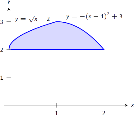
Figure \(\PageIndex{4}\): Graphing a region for Example \(\PageIndex{3}\).

Solution

We give two approaches to this problem. In the first approach, we notice that the region's "top" is defined by two different curves. On \([0,1]\), the top function is \(y=\sqrt{x}+2\); on \([1,2]\), the top function is \(y=-(x-1)^2+3\).

Thus we compute the area as the sum of two integrals:

\[\begin{align*} \text{Total Area} &= \int_0^1 \Big(\big(\sqrt{x}+2\big)-2\Big)\ dx + \int_1^2 \Big(\big(-(x-1)^2+3\big)-2\Big)\ dx \\[4pt] &= 2/3 + 2/3\\[4pt] &=4/3.\end{align*}\]

The second approach is clever and very useful in certain situations. We are used to viewing curves as functions of \(x\); we input an \(x\)-value and a \(y\)-value is returned. Some curves can also be described as functions of \(y\): input a \(y\)-value and an \(x\)-value is returned. We can rewrite the equations describing the boundary by solving for \(x\):

$$y=\sqrt{x}+2 \quad \Rightarrow\quad x=(y-2)^2\]

$$y=-(x-1)^2+3 \quad \Rightarrow \quad x=\sqrt{3-y}+1.\]

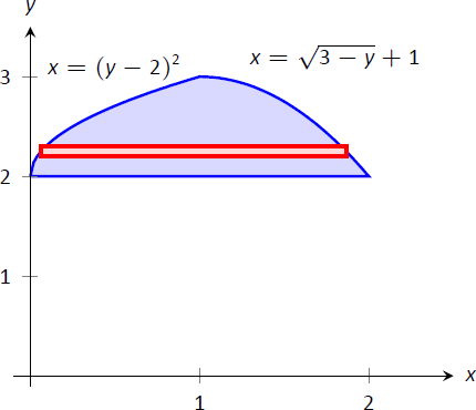
Figure \(\PageIndex{5}\):The region used in Example \(\PageIndex{3}\) with boundaries relabeled as functions of \(y\).

Figure \(\PageIndex{5}\) shows the region with the boundaries relabeled. A differential element, a horizontal rectangle, is also pictured. The width of the rectangle is a small change in \(y\): \(\Delta y\). The height of the rectangle is a difference in \(x\)-values. The "top" \(x\)-value is the largest value, i.e., the rightmost. The "bottom" \(x\)-value is the smaller, i.e., the leftmost. Therefore the height of the rectangle is

$$\big(\sqrt{3-y}+1\big) - (y-2)^2.\]

The area is found by integrating the above function with respect to \(y\) with the appropriate bounds. We determine these by considering the \(y\)-values the region occupies. It is bounded below by \(y=2\), and bounded above by \(y=3\). That is, both the "top" and "bottom" functions exist on the \(y\) interval \([2,3]\). Thus

\[\begin{align*}\text{Total Area} &= \int_2^3 \big(\sqrt{3-y}+1 - (y-2)^2\big)\ dy \\[4pt] &= \Big(-\dfrac23(3-y)^{3/2}+y-\dfrac13(y-2)^3\Big)\Big|_2^3 \\[4pt] &= 4/3.\end{align*}\]

This calculus--based technique of finding area can be useful even with shapes that we normally think of as "easy." Example \(\PageIndex{4}\) computes the area of a triangle. While the formula "\(\dfrac12\times\text{base}\times\text{height}\)" is well known, in arbitrary triangles it can be nontrivial to compute the height. Calculus makes the problem simple.

Example \(\PageIndex{4}\): Finding the area of a triangle

Compute the area of the regions bounded by the lines

\(y=x+1\), \(y=-2x+7\) and \(y=-\dfrac12x+\dfrac52\), as shown in Figure \(\PageIndex{6}\).

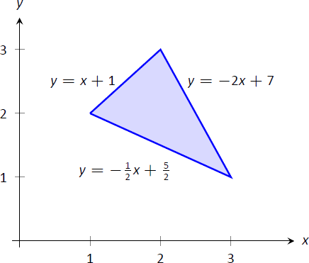
Figure \(\PageIndex{6}\): Graphing a triangular region in Example \(\PageIndex{4}\)

Solution

Recognize that there are two "top" functions to this region, causing us to use two definite integrals.

\[\begin{align*}\text{Total Area} &= \int_1^2\big((x+1)-(-\dfrac12x+\dfrac52)\big)\ dx + \int_2^3\big((-2x+7)-(-\dfrac12x+\dfrac52)\big)\ dx \\[4pt] &= 3/4+3/4\\[4pt] &=3/2.\end{align*}\]

We can also approach this by converting each function into a function of \(y\). This also requires 2 integrals, so there isn't really any advantage to doing so. We do it here for demonstration purposes.

The "top" function is always \(x=\dfrac{7-y}2\) while there are two "bottom" functions. Being mindful of the proper integration bounds, we have

\[\begin{align*} \text{Total Area} &= \int_1^2\big(\dfrac{7-y}2 - (5-2y)\big)\ dy + \int_2^3\big(\dfrac{7-y}2-(y-1)\big)\ dy \\[4pt] &= 3/4 + 3/4\\[4pt] &= 3/2.\end{align*}\]

Of course, the final answer is the same. (It is interesting to note that the area of all 4 subregions used is 3/4. This is coincidental.)

While we have focused on producing exact answers, we are also able to make approximations using the principle of Theorem \(\PageIndex{1}\). The integrand in the theorem is a distance ("top minus bottom"); integrating this distance function gives an area. By taking discrete measurements of distance, we can approximate an area using numerical integration techniques developed in Section \ref{sec:numerical_integration}. The following example demonstrates this.

Example \(\PageIndex{5}\): Numerically approximating area

To approximate the area of a lake, shown in Figure \(\PageIndex{7a}\), the "length" of the lake is measured at 200-foot increments as shown in Figure \(\PageIndex{7b}\), where the lengths are given in hundreds of feet. Approximate the area of the lake.

Solution

The measurements of length can be viewed as measuring "top minus bottom" of two functions. The exact answer is found by integrating \(\int_0^{12} \big(f(x)-g(x)\big)\ dx\), but of course we don't know the functions \(f\) and \(g\). Our discrete measurements instead allow us to approximate.

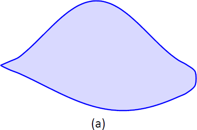
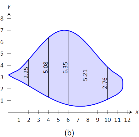
Figure \(\PageIndex{7}\): (a) A sketch of a lake, and (b) the lake with length measurements.

We have the following data points:

$$(0,0),\ (2,2.25),\ (4,5.08),\ (6,6.35),\ (8,5.21),\ (10,2.76),\ (12,0).\]

We also have that \(dx=\dfrac{b-a}{n} = 2\), so Simpson's Rule gives

\[\begin{align*}\text{Area}&\approx \dfrac{2}{3}\Big(1\cdot0+4\cdot2.25+2\cdot5.08+4\cdot6.35+2\cdot5.21+4\cdot2.76+1\cdot0\Big)\\[4pt] &= 44.01\overline{3} \ \text{units}^2.\end{align*}\]

Since the measurements are in hundreds of feet, units \(^2 = (100\ \text{ft})^2 = 10,000\ \text{ft}^2\), giving a total area of \(440,133\ \text{ft}^2\). (Since we are approximating, we'd likely say the area was about \(440,000\ \text{ft}^2\), which is a little more than 10 acres.)

In the next section we apply our applications--of--integration techniques to finding the volumes of certain solids.

Contributors and Attributions

• Gregory Hartman (Virginia Military Institute). Contributions were made by Troy Siemers and Dimplekumar Chalishajar of VMI and Brian Heinold of Mount Saint Mary's University. This content is copyrighted by a Creative Commons Attribution - Noncommercial (BY-NC) License. http://www.apexcalculus.com/

• Integrated by Justin Marshall.