4.11: Hyperbolic Functions

The hyperbolic functions appear with some frequency in applications, and are quite similar in many respects to the trigonometric functions. This is a bit surprising given our initial definitions.

Definition 4.11.1: Hyperbolic Cosines and Sines

The hyperbolic cosine is the function

$$\cosh x ={e^x +e^{-x }\over2},$$

and the hyperbolic sine is the function

$$\sinh x ={e^x -e^{-x}\over 2}.$$

Notice that $\cosh$ is even (that is, $\cosh(-x)=\cosh(x)$) while $\sinh$ is odd ($\sinh(-x)=-\sinh(x)$), and $\cosh x + \sinh x = e^x$. Also, for all $x$, $\cosh x >0$, while $\sinh x=0$ if and only if $e^x -e^{-x }=0$, which is true precisely when $x=0$.

Lemma 4.11.2

The range of $\cosh x$ is $[1,\infty)$.

Proof

Let $y= \cosh x$. We solve for $x$:

$$\eqalign{y&={e^x +e^{-x }\over 2}\cr 2y &= e^x + e^{-x }\cr 2ye^x &= e^{2x} + 1\cr 0 &= e^{2x}-2ye^x +1\cr e^{x} &= {2y \pm \sqrt{4y^2 -4}\over 2}\cr e^{x} &= y\pm \sqrt{y^2 -1}\cr}$$

From the last equation, we see $y^2 \geq 1$, and since $y\geq 0$, it follows that $y\geq 1$.

Now suppose $y\geq 1$, so $y\pm \sqrt{y^2 -1}>0$. Then $x = \ln(y\pm \sqrt{y^2 -1})$ is a real number, and $y =\cosh x$, so $y$ is in the range of $\cosh(x)$.

$\square$

Definition 4.11.3: Hyperbolic Tangent and Cotangent

The other hyperbolic functions are

$$\eqalign{\tanh x &= {\sinh x\over\cosh x}\cr \coth x &= {\cosh x\over\sinh x}\cr \text{sech} x &= {1\over\cosh x}\cr \text{csch} x &= {1\over\sinh x}\cr}$$

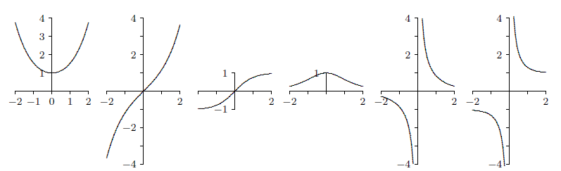
The domain of $\coth$ and $\text{csch}$ is $x\neq 0$ while the domain of the other hyperbolic functions is all real numbers. Graphs are shown in Figure $\PageIndex{1}$

Figure $\PageIndex{1}$: The hyperbolic functions.

Certainly the hyperbolic functions do not closely resemble the trigonometric functions graphically. But they do have analogous properties, beginning with the following identity.

Theorem 4.11.4

For all $x$ in $\mathbb{R}$, $\cosh ^2 x -\sinh ^2 x = 1$.

Proof

The proof is a straightforward computation:

$$\cosh ^2 x -\sinh ^2 x = {(e^x +e^{-x} )^2\over 4} -{(e^x -e^{-x} )^2\over 4}= {e^{2x} + 2 + e^{-2x } - e^{2x } + 2 - e^{-2x}\over 4}= {4\over 4} = 1.$$

$\square$

This immediately gives two additional identities:

$$1-\tanh^2 x =\text{sech}^2 x\qquad\hbox{and}\qquad \coth^2 x - 1 =\text{csch}^2 x.$$

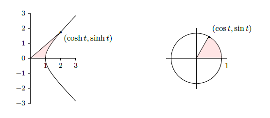
The identity of the theorem also helps to provide a geometric motivation. Recall that the graph of $x^2 -y^2 =1$ is a hyperbola with asymptotes $x=\pm y$ whose $x$-intercepts are $\pm 1$. If $(x,y)$ is a point on the right half of the hyperbola, and if we let $x=\cosh t$, then $y=\pm\sqrt{x^2-1}=\pm\sqrt{\cosh^2x-1}=\pm\sinh t$. So for some suitable $t$, $\cosh t$ and $\sinh t$ are the coordinates of a typical point on the hyperbola. In fact, it turns out that $t$ is twice the area shown in the first graph of Figure $\PageIndex{2}$. Even this is analogous to trigonometry; $\cos t$ and $\sin t$ are the coordinates of a typical point on the unit circle, and $t$ is twice the area shown in the second graph of Figure $\PageIndex{2}$.

Figure $\PageIndex{2}$: Geometric definitions of sin, cos, sinh, cosh: $t$ is twice the shaded area in each figure.

Given the definitions of the hyperbolic functions, finding their derivatives is straightforward. Here again we see similarities to the trigonometric functions.

Theorem 4.11.5

${d\over dx}\cosh x=\sinh x$ and \thmrdef{thm:hyperbolic derivatives} ${d\over dx}\sinh x = \cosh x$.

Proof

$${d\over dx}\cosh x= {d\over dx}{e^x +e^{-x}\over 2} = {e^x- e^{-x}\over 2} =\sinh x,$$

and

$${d\over dx}\sinh x = {d\over dx}{e^x -e^{-x}\over 2} = {e^x +e^{-x }\over 2} =\cosh x.$$

$\square$

Since $\cosh x > 0$, $\sinh x$ is increasing and hence injective, so $\sinh x$ has an inverse, $\text{arcsinh} x$. Also, $\sinh x > 0$ when $x>0$, so $\cosh x$ is injective on $[0,\infty)$ and has a (partial) inverse, $\text{arccosh} x$. The other hyperbolic functions have inverses as well, though $\text{arcsech} x$ is only a partial inverse. We may compute the derivatives of these functions as we have other inverse functions.

Theorem 4.11.6

${d\over dx}\text{arcsinh} x = {1\over\sqrt{1+x^2}}$.

Proof

Let $y=\text{arcsinh} x$, so $\sinh y=x$. Then

$${d\over dx}\sinh y = \cosh(y)\cdot y' = 1,$$

and so

$$y' ={1\over\cosh y} ={1\over\sqrt{1 +\sinh^2 y}} = {1\over\sqrt{1+x^2}}.$$

$\square$

The other derivatives are left to the exercises.

Contributors

• David Guichard (Whitman College)

• Integrated by Justin Marshall.