10.4: Applications of the Logarithm

Learning Objectives

1. Describe the relationships between properties of \(e^{x}\) and properties of its inverse \(\ln (x)\), and master manipulations of expressions involving both.
2. Use logarithms for base conversions.
3. Use logarithms to solve equations involving the exponential function, i.e. solve \(A=e^{b t}\) for \(t\).)
4. Given a relationship such as \(y=a x^{b}\), show that \(\ln (y)\) is related linearly to \(\ln (x)\), and use data points for \((x, y)\) to determine the values of \(a\) and \(b\).

Using the logarithm for base conversion

The logarithm is helpful in changing an exponential function from one base to another. We give some examples here.

Example 10.9

Rewrite \(y=2^{x}\) in terms of base \(e\).

Solution

We apply ln and then exponentiate the result. Manipulations of exponents and logarithms lead to the desired results as follows:

\[\begin{gathered} y=2^{x} \Rightarrow \ln (y)=\ln \left(2^{x}\right)=x \ln (2) . \\ e^{\ln (y)}=e^{x \ln (2)} \Rightarrow y=e^{x \ln (2)} . \end{gathered} \nonumber \]

We find (using a calculator) that \(\ln (2)=0.6931 \ldots\) This coincides with the value we computed earlier for \(C_{2}\) in Example 10.4, so we have

\[y=e^{k x} \quad \text { where } \quad k=\ln (2)=0.6931 \ldots \nonumber \]

Mastered Material Check

23. Why might one base be preferred over another?

Example 10.10

Find the derivative of \(y=2^{x}\).

Solution

In Example \(10.9\) we expressed this function in the alternate form

\[y=2^{x}=e^{k x} \quad \text { with } \quad k=\ln (2) . \nonumber \]

From Example \(10.7\) we have

\[\frac{d y}{d x}=k e^{k x}=\ln (2) e^{\ln (2) x}=\ln (2) 2^{x} . \nonumber \]

Through the above base conversion and chain rule, we relate the constant \(C_{2}\) in Example \(10.4\) to the natural logarithm of 2: \(C_{2}=\ln (2)\).

The logarithm helps to solve exponential equations

Equations involving the exponential function can sometimes be simplified and solved using the logarithm. We provide a few examples of this kind.

Example 10.11

Find zeros of the function \(y=f(x)=e^{2 x}-e^{5 x^{2}}\).

Solution

We seek values of \(x\) for which \(f(x)=e^{2 x}-e^{5 x^{2}}=0\). We write

\[e^{2 x}-e^{5 x^{2}}=0 \Rightarrow e^{2 x}=e^{5 x^{2}} \quad \Rightarrow \quad \frac{e^{5 x^{2}}}{e^{2 x}}=1 \quad \Rightarrow \quad e^{5 x^{2}-2 x}=1 . \nonumber \]

Taking logarithm of both sides, and using the facts that \(\ln \left(e^{5 x^{2}-2 x}\right)=5 x^{2}-2 x\) and \(\ln (1)=0\), we obtain

\[e^{5 x^{2}-2 x}=1 \quad \Rightarrow \quad 5 x^{2}-2 x=0 \quad \Rightarrow \quad x=0, \frac{2}{5} . \nonumber \]

We see that the logarithm is useful in the last step of isolating \(x\), after simplifying the exponential expressions appearing in the equation.

Andromeda Strain, revisited. In Section \(10.1\) we posed the question: how long does it take for the Andromeda strain population to attain a size of \(6 \cdot 10^{39}\) cells, i.e. to grow to an Earth-sized colony? We now solve this problem using the continuous exponential function and the logarithm.

Recall that the bacterial doubling time is \(20 \mathrm{~min}\). If time is measured in minutes, the number, \(B(t)\) of bacteria at time \(t\) could be described by the smooth function:

\[B(t)=2^{t / 20} . \nonumber \]

Mastered Material Check

24. Verify that \(B(t)\) agrees with Figure \(10.1\) and give powers of 2 at \(t=20,40,60,80, \ldots\) minutes.
25. When, in general, will \(B(t)\) give a power of 2 ?

Example 10.12

(The Andromeda strain) Starting from a single cell, how long does it take for an E. coli colony to reach size of \(6 \cdot 10^{39}\) cells by doubling every 20 minutes?

Solution

We compute the time it takes by solving for \(t\) in \(B(t)=6 \cdot 10^{39}\), as shown below.

\[\begin{gathered} 6 \cdot 10^{39}=2^{t / 20} \Rightarrow \ln \left(6 \cdot 10^{39}\right)=\ln \left(2^{t / 20}\right) \\ \ln (6)+39 \ln (10)=\frac{t}{20} \ln (2) \end{gathered} \nonumber \]

Solving for \(t\),

\[t=20 \frac{\ln (6)+39 \ln (10)}{\ln (2)}=20 \frac{1.79+39(2.3)}{0.693}=2643.4 \mathrm{~min}=\frac{2643.27}{60} \mathrm{hr} . \nonumber \]

Hence, it takes 44 hours (but less than 2 days) for the colony to "grow to the size of planet Earth" (assuming the implausible scenario of unlimited growth).

Example 10.13 (Using base \(e\))

Express the number of bacteria in terms of base e (for practice with base conversions).

Solution

Given \(B(t)=2^{t / 20}\) is the number of bacteria at time \(t\), we proceed as follows:

\[\begin{aligned} & \quad B(t)=2^{t / 20} \quad \Rightarrow \quad \ln (B(t))=\frac{t}{20} \ln (2) \\ & e^{\ln (B(t))}=e^{\frac{t}{20} \ln (2)} \Rightarrow B(t)=e^{k t} \quad \text { where } \quad k=\frac{\ln (2)}{20} \text { per min. } \end{aligned} \nonumber \]

The constant \(k\) has units of \(1 /\) time. We refer to \(k\) as the growth rate of the bacteria. We observe that this constant can be written as:

\[k=\frac{\ln (2)}{\text { doubling time }} . \nonumber \]

As we see next, this approach is helpful in scientific applications.

Logarithms help plot data that varies on large scale

Living organisms come in a variety of sizes, from the tiniest cells to the largest whales. Comparing attributes across species of vastly different sizes poses a challenge, as visualizing such data on a simple graph obscures both extremes.

Suppose we wish to compare the physiology of organisms of various sizes, from that of a mouse to that of an elephant. An example of such data for metabolic rate versus mass of the animal is shown in Table 10.4.

Table 10.4: Animals of various sizes (mass \(M\) in \(\mathrm{gm}\) ) have widely different basal metabolic rates (BMR, generally measured in terms of oxygen consumption rate, i.e. ml \(\mathrm{O}_{2}\) consumed per hr).

animal	body weight \(M(\mathrm{gm})\)	basal metabolic rate (BMR)
mouse	25	1580
rat	226	873
rabbit	2200	466
dog	11700	318
man	70000	202
horse	700000	106

A log-log plot of this data is shown in Figure 10.8.

Figure 10.8: A log-log plot of the data in Table 10.4, showing \(\ln (\mathrm{BMR})\) versus \(\ln (M)\).

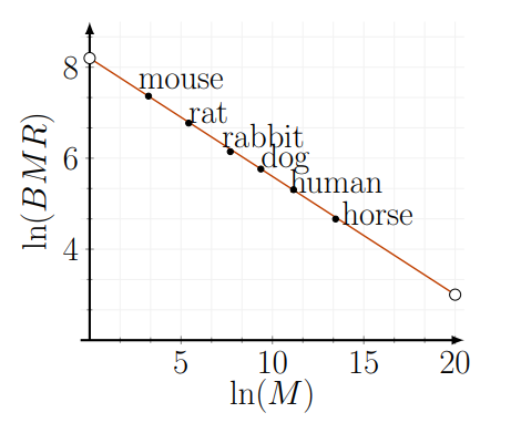
It would be hard to see all data points clearly on a regular graph. For this reason, it is helpful to use logarithmic scaling for either or both variables. We show an example of this kind of log-log plot, where both axes use logarithmic scales, in Figure 10.8.

In allometry, it is conjectured that such data fits some power function of the form

\[y \approx a x^{b}, \text { where } a, b>0 \]

Note: this is not an exponential function, but a power function with power \(b\) and coefficient \(a\).

Finding the allometric constants \(a\) and \(b\) using the graph in Fig \(10.8\) is now explained.

Example 10.14 (Log transformation)

Define \(Y=\ln (y)\) and \(X=\ln (x)\). Show that (10.4.1) can be rewritten as a linear relationship between \(Y\) and \(X\).

Solution

We have

\[Y=\ln (y)=\ln \left(a x^{b}\right)=\ln (a)+\ln \left(x^{b}\right)=\ln (a)+b \ln (x)=A+b X, \nonumber \]

where \(A=\ln (a)\). Thus, we have shown that \(X\) and \(Y\) are related linearly:

\[Y=A+b X, \quad \text { where } A=\ln (a) . \nonumber \]

This is the equation of a straight line with slope \(b\) and \(Y\) intercept \(A\).

Mastered Material Check

26. Use software to plot the data given in Table 10.4. Why is it so hard to plot on a regular graph?

Example 10.15 (Finding the constants)

Use the straight line superimposed on the data in Figure \(10.8\) to estimate the values of the constants \(a\) and \(b\).

Solution

We use the straight line that has been fitted to the data in Figure 10.8. The \(Y\) intercept is roughly 8.2. The line goes approximately through \((20,3)\) and \((0,8.2)\) (open dots on plot) so its slope is \(\approx(3-\) 8.2) \(/ 20=-0.26\). According to the relationship we found in Example 10.14,

\[8.2=A=\ln (a) \Rightarrow a=e^{8.2}=3640, \quad \text { and } \quad b=-0.26 . \nonumber \]

Thus, reverting to the original allometric relationship leads to

\[y=a x^{b}=3640 x^{-0.26}=\frac{3640}{x^{0.26}} . \nonumber \]

From this we see that the metabolic rate \(y\) decreases with the size \(x\) of the animal, as indicated by the data in Table 10.4.