In this section we will briefly discuss some applications of multiple integrals in the field of probability theory. In particular we will see ways in which multiple integrals can be used to calculate probabilities and expected values.
Probability
Suppose that you have a standard six-sided (fair) die, and you let a variable represent the value rolled. Then the probability of rolling a 3, written as , is 1 6 , since there are six sides on the die and each one is equally likely to be rolled, and hence in particular the 3 has a one out of six chance of being rolled. Likewise the probability of rolling at most a 3, written as , is , since of the six numbers on the die, there are three equally likely numbers (1, 2, and 3) that are less than or equal to 3. Note that:
We call a discrete random variable on the sample space (or probability space) consisting of all possible outcomes. In our case, . An event is a subset of the sample space. For example, in the case of the die, the event is the set .
Now let be a variable representing a random real number in the interval . Note that the set of all real numbers between 0 and 1 is not a discrete (or countable) set of values, i.e. it can not be put into a one-to-one correspondence with the set of positive integers. In this case, for any real number in , it makes no sense to consider since it must be 0 (why?). Instead, we consider the probability , which is given by . The reasoning is this: the interval has length 1, and for in the interval has length . So since represents a random number in , and hence is uniformly distributed over , then
We call a continuous random variable on the sample space. An event is a subset of the sample space. For example, in our case the event is the set .
In the case of a discrete random variable, we saw how the probability of an event was the sum of the probabilities of the individual outcomes comprising that event (e.g. in the die example). For a continuous random variable, the probability of an event will instead be the integral of a function, which we will now describe.
Let be a continuous real-valued random variable on a sample space in . For simplicity, let . Define the distribution function of as
Suppose that there is a nonnegative, continuous real-valued function on such that
and
Then we call the probability density function (or . for short) for . We thus have
Also, by the Fundamental Theorem of Calculus, we have
Example : Uniform Distribution
Let represent a randomly selected real number in the interval . We say that has the uniform distribution on , with distribution function
and probability density function
In general, if represents a randomly selected real number in an interval , then has the uniform distribution function
Example : Standard Normal Distribution
A famous distribution function is given by the standard normal distribution, whose probability density function is
This is often called a “bell curve”, and is used widely in statistics. Since we are claiming that is a , we should have
by Equation , which is equivalent to
We can use a double integral in polar coordinates to verify this integral. First,
since the same function is being integrated twice in the middle equation, just with different variables. But using polar coordinates, we see that
and so
In addition to individual random variables, we can consider jointly distributed random variables. For this, we will let be three real-valued continuous random variables defined on the same sample space in (the discussion for two random variables is similar). Then the joint distribution function is given by
If there is a nonnegative, continuous real-valued function on such that
and
then we call the joint probability density function (or joint p.d.f. for short) for . In general, for , we have
with the symbols interchangeable in any combination. A triple integral, then, can be thought of as representing a probability (for a function which is a ).
Example
Let be real numbers selected randomly from the interval . What is the probability that the equation has at least one real solution ?
Solution
We know by the quadratic formula that there is at least one real solution if . So we need to calculate . We will use three jointly distributed random variables to do this. First, since we have
where the last relation holds for all such that
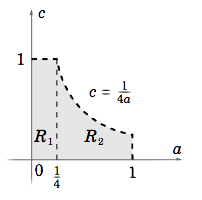
Considering as real variables, the region in the -plane where the above relation holds is given by , which we can see is a union of two regions and , as in Figure .
Figure : Region
Now let be continuous random variables, each representing a randomly selected real number from the interval (think of representing , respectively). Then, similar to how we showed that is the of the uniform distribution on , it can be shown that in (0 elsewhere) is the joint . Now,
so this probability is the triple integral of as b varies from to 1 and as varies over the region . Since can be divided into two regions , then the required triple integral can be split into a sum of two triple integrals, using vertical slices in :
In other words, the equation has about a 25% chance of being solved!
Expectation Value
The expectation value (or expected value) of a random variable can be thought of as the “average” value of as it varies over its sample space. If is a discrete random variable, then
with the sum being taken over all elements of the sample space. For example, if represents the number rolled on a six-sided die, then
is the expected value of , which is the average of the integers 1−6.
If is a real-valued continuous random variable with p.d.f. , then
For example, if has the uniform distribution on the interval , then its p.d.f. is
and so
For a pair of jointly distributed, real-valued continuous random variables and with joint p.d.f. , the expected values of are given by
respectively.
Example
If you were to pick random real numbers from the interval , what are the expected values for the smallest and largest of those numbers?
Solution
Let be continuous random variables, each representing a randomly selected real number from , i.e. each has the uniform distribution on . Define random variables by
Then it can be shown that the joint p.d.f. of is
Thus, the expected value of is
and similarly (see Exercise 3) it can be shown that
So, for example, if you were to repeatedly take samples of random real numbers from , and each time store the minimum and maximum values in the sample, then the average of the minimums would approach and the average of the maximums would approach as the number of samples grows. It would be relatively simple (see Exercise 4) to write a computer program to test this.