Green's Theorem

A Little Topology

Before stating the big theorem of the day, we first need to present a few topological ideas: simple connected regions and orientation. Consider a closed curve $C$ in $\mathbb{R}^2$ defined parametrically by

$$\textbf{r}(t) = x(t)\hat{\textbf{i}} + y(t)\hat{\textbf{j}} \nonumber$$

with $a \leq t \leq b$. We say $C$ is simple if it does not intersect itself. A curve intersects itself if

$$\textbf{r}(u) = \textbf{r}(v) \nonumber$$

for two distinct values $u$ and $v$. A circle is a simple curve while a figure eight is not simple.

A region is called simply connected if it boundary is a single simple closed curve. Another way of thinking about simply connected regions is that their complement (the space minus the region) consists of only one piece. Below are examples of simply connected and non-simply connected regions.

Our final topological definition is orientation. We have seen that if we traverse a curve in the opposite direction, then the line integral will be the negative of the original. We want to have a way to define a positive orientation. We define it as follows.

Definition: Orientation

Let $R$ be a simply connected region with boundary curve $C$. Then $C$ is called positively oriented if facing the direction that the curve is sketched, the region lies to the left of the curve. Otherwise the curve is said to be negatively oriented.

One way to remember this is to recall that in the standard unit circle angles are measures counterclockwise, that is traveling around the circle you will see the center on your left.

Green's Theorem

We have seen that if a vector field

$$\textbf{F} = M \textbf{i} + N\textbf{j} \nonumber$$

has the property that

$$N_x - M_y = 0 \nonumber$$

then the line integral over any smooth closed curve is zero. What can we do if the above quantity is nonzero. Green's theorem states that the line integral is equal to the double integral of this quantity over the enclosed region.

Green's Theorem

Let $R$ be a simply connected region with smooth boundary $C$, oriented positively and let $M$ and $N$ have continuous partial derivatives in an open region containing $R$, then

$$\oint_c M \, dx + N\, dy = \iint _R \left(N_x-M_y \right) \, dy\,dx \nonumber$$

Proof

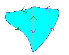
First we can assume that the region is both vertically and horizontally simple. Otherwise we can carefully cut the region into parts so that each of the parts are both vertically simple and horizontally simple. Below is an example of such a cut. Notice that the line where the regions is cut is drawn once upwards and once downwards. Thus the two line integrals over this line will cancel each other out.

We can assume that the region is as in the figure below

We will show that

$$\oint_c N\;dy = \iint_R N_x \;dx\;dy \label{eq45}$$

The proof for the $M$ part is similar. We will compute both sides and show they are the same. First we break the curve into its left and right half. Call the left half $C_1$ and the right half $C_2$. We have

$$\begin{align} \oint_c N \; dy &= \int_{C_1}N \; dy + \int_{C_2}N \; dy \nonumber \\[4pt] &= \int_a^b N(g_1(y),y)dy + \int_a^b N(g_2(y),y) dy \nonumber \\[4pt] &= \int_a^b [N(g_2 (y),y)-N(g_1(y),y) ]\; dy \label{eq50}\end{align}$$

Now we show that the double integral leads to the same expression. We have

$$\begin{align} \iint_R N_x \;dy\,dx &= \int_a^b \int_{g_1(y)}^{g_2(y)} N_x \; dx\,dy \nonumber \\[4pt] &= \int_a^b [N(x,y)]_{g_1(y)}^{g_2(y)} dy \nonumber\\[4pt] &= \int _a^b [N(g_2(y),y)-N(g_1(y),y)]dy \label{eq51} \end{align}$$

both Equation $\ref{eq50}$ and $\ref{eq51}$ are equal, therefore Equation $\ref{eq45}$ is true.

$\square$

Example $\PageIndex{1}$: Using Green's Theorem

Determine the work done by the force field

$$\textbf{F} = (x - xy) \hat{\textbf{i}} + y^2 \textbf{j} \nonumber$$

when a particle moves counterclockwise along the rectangle with vertices $(0,0)$, $(4,0)$, $(4,6)$, and $(0,6)$.

Solution

We could do this with a line integral, but this would involve four parameterizations (one for each side of the rectangle). Instead, we use Green's Theorem. We find

$$N_x - M_y = 0 - (-x) = x \nonumber$$

The region is just a rectangle, so the limits are the constants. We have

$$\begin{align*} \int_0^4 \int_0^6 x \; dydx &= \int_0^4 [xy]_0^6 \\[4pt] &= \int_0^4 6x \; dx \\[4pt] &= [3x^2]_0^4 \\[4pt] &= 48 \end{align*}$$

Example $\PageIndex{2}$

Calculate the line integral

$$\int_C (3-x) \,dx + (x-y) \,dy\nonumber$$

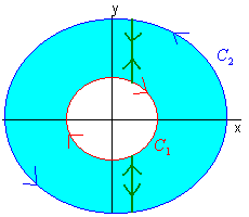
where $C$ is the union of the unit circle centered at the origin oriented negatively and the circle of radius 2 centered at the origin oriented positively.

Solution

We cannot use Green's Theorem directly, since the region is not simply connected. However, if we think of the region as being the union its left and right half, then we see that the extra cuts cancel each other out.

In this light we can use Green's Theorem on each piece. We have

$$N_x - M_y = 1 - 0 = 1 \nonumber$$

Hence the line integral is just the double integral of 1, which is the area of the region. This area is

$$\pi(2^2 - 1^2) = 4\pi \nonumber$$

Green's Theorem and Area

The example above showed that if

$$N_x - M_y = 1 \nonumber$$

then the line integral gives the area of the enclosed region. There are three special vector fields, among many, where this equation holds. We state the following theorem which you should be easily able to prove using Green's Theorem.

Using Green's Theorem to Find Area

Let $R$ be a simply connected region with positively oriented smooth boundary $C$. Then the area of $R$ is given by each of the following line integrals.

1. $\displaystyle \oint_C x\,dy$
2. $\displaystyle \oint_c -y\, dx$
3. $\displaystyle \frac{1}{2} \oint x \, dy - y \, dx$

Example $\PageIndex{3}$

Use the third part of the area formula to find the area of the ellipse

$$\dfrac{x^2}{4} + \dfrac{y^2}{9} =1 \nonumber$$

Solution

To compute the line integral, we parameterize the curve

$$\begin{align*} \textbf{r}(t) &= 2 \cos t \hat{\textbf{i}} + 3 \sin t \hat{\textbf{j}} \\[4pt] \textbf{r}'(t) &= -2 \sin t \hat{\textbf{i}} + 3 \cos t \hat{\textbf{j}} \end{align*}$$

We have

$$\begin{align*} \dfrac{1}{2}\int_C x \; dy - y \; dx &= \dfrac{1}{2}\int_0^{2\pi} [(2 \cos t)(3 \cos t)- (3 \sin t)(-2 \sin t)] dt \\[4pt] &= \dfrac{1}{2}\int_0^{2\pi} (6 \cos^2 t + 6 \sin^2 t)dt \\[4pt] &= \dfrac{1}{2}\int_0^{2\pi} 6 \; dt \\[4pt] &= 6 \pi \end{align*}\nonumber$$

Contributors and Attributions

• Larry Green (Lake Tahoe Community College)