4.2: Best Affine Approximations

Best affine approximations

The following definitions should look very familiar.

Definition \(\PageIndex{1}\)

Suppose \(f: \mathbb{R}^{m} \rightarrow \mathbb{R}^{n}\) is defined on an open ball containing the point \(\mathbf{c}\). We call an affine function \(A: \mathbb{R}^{m} \rightarrow \mathbb{R}^{n}\) the best affine approximation to \(f\) at \(\mathbf{c}\) if (1) \(A(\mathbf{c})=f(\mathbf{c})\) and (2) \(\|R(\mathbf{h})\|\) is \(o(\mathbf{h})\), where

\[ R(\mathbf{h})=f(\mathbf{c}+\mathbf{h})-A(\mathbf{c}+\mathbf{h}) . \]

Suppose \(A: \mathbb{R}^{n} \rightarrow \mathbb{R}^{n}\) is the best affine approximation to \(f\) at \(\mathbf{c}\). Then, from our work in Section 1.5, there exists an \(n \times m\) matrix \(M\) and a vector \(\mathbf{b}\) in \(\mathbb{R}^n\) such that

\[ A(\mathbf{x})=M \mathbf{x}+\mathbf{b} \]

for all \(\mathbf{x}\) in \(\mathbb{R}^m\). Moreover, the condition \(A(\mathbf{c})=f(\mathbf{c})\) implies \(f(\mathbf{c})=M \mathbf{c}+\mathbf{b}\), and so \(\mathbf{b}=f(\mathbf{c})-M \mathbf{c}\). Hence we have

\[ A(\mathbf{x})=M \mathbf{x}+f(\mathbf{c})-M \mathbf{c}=M(\mathbf{x}-\mathbf{c})+f(\mathbf{c}) \label{4.2.3} \]

for all \(\mathbf{x}\) in \(\mathbb{R}^m\). Thus to find the best affine approximation we need only identify the matrix \(M\) in (\(\ref{4.2.3}\)).

Definition \(\PageIndex{2}\)

Suppose \(f: \mathbb{R}^{m} \rightarrow \mathbb{R}^{n}\) is defined on an open ball containing the point \(\mathbf{c}\). If \(f\) has a best affine approximation at \(\mathbf{c}\), then we say \(f\) is differentiable at \(\mathbf{c}\). Moreover, if the best affine approximation to \(f\) at \(\mathbf{c}\) is given by

\[ A(\mathbf{x})=M(\mathbf{x}-\mathbf{c})+f(\mathbf{c}) , \]

then we call \(M\) the derivative of \(f\) at \(\mathbf{c}\) and write \(D f(\mathbf{c})=M\).

Now suppose \(f: \mathbb{R}^{m} \rightarrow \mathbb{R}^{n}\) and \(A\) is an affine function with \(A(\mathbf{c})=f(\mathbf{c})\). Let \(f_k\) and \(A_k\) be the \(k\)th coordinate functions of \(f\) and \(A\), respectively, for \(k=1,2, \ldots, n\), and let \(R\) be the remainder function

\[ \begin{aligned}
R(\mathbf{h}) &=f(\mathbf{c}+\mathbf{h})-A(\mathbf{c}+\mathbf{h}) \\
&=\left(f_{1}(\mathbf{c}+\mathbf{h})-A_{1}(\mathbf{c}+\mathbf{h}), f_{2}(\mathbf{c}+\mathbf{h})-A_{2}(\mathbf{c}+\mathbf{h}), \ldots, f_{n}(\mathbf{c}+\mathbf{h})-A_{n}(\mathbf{c}+\mathbf{h})\right).
\end{aligned} \]

Then

\[ \frac{R(\mathbf{h})}{\|\mathbf{h}\|}=\left(\frac{f_{1}(\mathbf{c}+\mathbf{h})-A_{1}(\mathbf{c}+\mathbf{h})}{\|\mathbf{h}\|}, \frac{f_{2}(\mathbf{c}+\mathbf{h})-A_{2}(\mathbf{c}+\mathbf{h})}{\|\mathbf{h}\|}, \ldots, \frac{f_{n}(\mathbf{c}+\mathbf{h})-A_{n}(\mathbf{c}+\mathbf{h})}{\|\mathbf{h}\|}\right) , \nonumber \]

and so

\[ \lim _{\mathbf{h} \rightarrow \mathbf{0}} \frac{\| R(\mathbf{h} \|}{\|\mathbf{h}\|}=0 , \]

that is, \(A\) is the best affine approximation to \(f\) at \(\mathbf{c}\), if and only if

\[ \lim _{\mathbf{h} \rightarrow \mathbf{0}} \frac{f_{k}(\mathbf{c}+\mathbf{h})-A_{k}(\mathbf{c}+\mathbf{h})}{\|\mathbf{h}\|}=0 \label{4.2.6} \]

for \(k=1,2, \ldots, n\). But (\(\ref{4.2.6}\)) is the statement that \(A_k\) is the best affine approximation to \(f_k\) at \(\mathbf{c}\). In other words, \(A\) is the best affine approximation to \(f\) at \(\mathbf{c}\) if and only if \(A_k\) is the best affine approximation to \(f_k\) at \(\mathbf{c}\) for \(k=1,2, \ldots, n\). This result has many interesting consequences.

Proposition \(\PageIndex{1}\)

If \(f_{k}: \mathbb{R}^{m} \rightarrow \mathbb{R}\) is the \(k\)th coordinate function of \(f: \mathbb{R}^{m} \rightarrow \mathbb{R}^{n}\), then \(f\) is differentiable at a point \(\mathbf{c}\) if and only if \(f_k\) is differentiable at \(\mathbf{c}\) for \(k=1,2, \ldots, n\).

Definition \(\PageIndex{3}\)

If \(f_{k}: \mathbb{R}^{m} \rightarrow \mathbb{R}\) is the \(k\)th coordinate function of \(f: \mathbb{R}^{m} \rightarrow \mathbb{R}^{n}\), then we say \(f\) is \(C^1\) on an open set \(U\) if \(f_k\) is \(C^1\) on \(U\) for \(k=1,2, \ldots, n\).

Putting our results in Section 3.3 together with the previous proposition and definition, we have the following basic result.

Theorem \(\PageIndex{1}\)

If \(f: \mathbb{R}^{m} \rightarrow \mathbb{R}^{n}\) is \(C^1\) on an open ball containing the point \(\mathbf{c}\), then \(f\) is differentiable at \(\mathbf{c}\).

Suppose \(f: \mathbb{R}^{m} \rightarrow \mathbb{R}^{n}\) is differentiable at \(\mathbf{c}=\left(c_{1}, c_{2}, \ldots, c_{m}\right)\) with best affine approximation \(A\) and \(f_{k}: \mathbb{R}^{m} \rightarrow \mathbb{R}\) and \(A_{k}: \mathbb{R}^{m} \rightarrow \mathbb{R}\) are the coordinate functions of \(f\) and \(A\), respectively, for \(k=1,2, \ldots, n\). Since \(A_k\) is the best affine approximation to \(f_k\) at \(\mathbf{c}\), we know from Section 3.3 that

\[ A_{k}(\mathbf{x})=\nabla f_{k}(\mathbf{c}) \cdot(\mathbf{x}-\mathbf{c})+f_{k}(\mathbf{c}) \]

for all \(\mathbf{x}\) in \(\mathbb{R}^m\). Hence, writing the vectors as column vectors, we have

\[ \begin{align}
A(\mathbf{x})=&\left[\begin{array}{c}
A_{1}(\mathbf{x}) \\
A_{2}(\mathbf{x}) \\
\vdots \\
A_{n}(\mathbf{x})
\end{array}\right] \nonumber \\
=&\left[\begin{array}{cccc}
\nabla f_{1}(\mathbf{c}) \cdot(\mathbf{x}-\mathbf{c})+f_{1}(\mathbf{c}) \\
\nabla f_{2}(\mathbf{c}) \cdot(\mathbf{x}-\mathbf{c})+f_{2}(\mathbf{c}) \\
\vdots \\
\nabla f_{n}(\mathbf{c}) \cdot(\mathbf{x}-\mathbf{c})+f_{n}(\mathbf{c})
\end{array}\right] \nonumber \\
=&\left[\begin{array}{cccc}
\frac{\partial}{\partial x_{1}} f_{1}(\mathbf{c}) & \frac{\partial}{\partial x_{2}} f_{1}(\mathbf{c}) & \cdots & \frac{\partial}{x_{m}} f_{1}(\mathbf{c}) \\
\frac{\partial}{\partial x_{1}} f_{2}(\mathbf{c}) & \frac{\partial}{\partial x_{2}} f_{2}(\mathbf{c}) & \cdots & \frac{\partial}{x_{m}} f_{2}(\mathbf{c}) \\
\vdots & \vdots & \ddots & \vdots \\
\frac{\partial}{\partial x_{1}} f_{n}(\mathbf{c}) & \frac{\partial}{\partial x_{2}} f_{n}(\mathbf{c}) & \cdots & \frac{\partial}{x_{m}} f_{n}(\mathbf{c})
\end{array}\right]\left[\begin{array}{c}
x_{1}-c_{1} \\
x_{2}-c_{2} \\
\vdots \\
x_{m}-c_{m}
\end{array}\right]+\left[\begin{array}{c}
f_{1}(\mathbf{c}) \\
f_{2}(\mathbf{c}) \\
\vdots \\
f_{m}(\mathbf{c})
\end{array}\right] . \label{4.2.8}
\end{align} \]

It follows that the \(n \times m \) matrix in (\(\ref{4.2.8}\)) is the derivative of \(f\).

Theorem \(\PageIndex{2}\)

If \(f: \mathbb{R}^{m} \rightarrow \mathbb{R}^{n}\) is differentiable at a point \(\mathbf{c}\), then the derivative of \(f\) at \(\mathbf{c}\) is given by

\[ D f(\mathbf{c})=\left[\begin{array}{cccc}
\frac{\partial}{\partial x_{1}} f_{1}(\mathbf{c}) & \frac{\partial}{\partial x_{2}} f_{1}(\mathbf{c}) & \cdots & \frac{\partial}{x_{m}} f_{1}(\mathbf{c}) \\
\frac{\partial}{\partial x_{1}} f_{2}(\mathbf{c}) & \frac{\partial}{\partial x_{2}} f_{2}(\mathbf{c}) & \cdots & \frac{\partial}{x_{m}} f_{2}(\mathbf{c}) \\
\vdots & \vdots & \ddots & \vdots \\
\frac{\partial}{\partial x_{1}} f_{n}(\mathbf{c}) & \frac{\partial}{\partial x_{2}} f_{n}(\mathbf{c}) & \cdots & \frac{\partial}{x_{m}} f_{n}(\mathbf{c})
\end{array}\right] . \label{4.2.9} \]

We call the matrix in (\(\ref{4.2.9}\)) the Jacobian matrix of \(f\), after the German mathematician Carl Gustav Jacob Jacobi (1804-1851). Note that we have seen this matrix before in our discussion of change of variables in integrals in Section 3.7.

Example \(\PageIndex{1}\)

Consider the function \(f: \mathbb{R}^{3} \rightarrow \mathbb{R}^{2}\) defined by

\[ f(x, y, z)=(x y z, 3 x-2 y z) . \nonumber \]

The coordinate functions of \(f\) are

\[ f_{1}(x, y, z)=x y z \nonumber \]

and

\[ f_{2}(x, y, z)=3 x-2 y z \text {. } \nonumber \]

Now

\[ \nabla f_{1}(x, y, z)=(y z, x z, x y) \nonumber \]

and

\[ \nabla f_{2}(x, y, z)=(3,-2 z,-2 y) , \nonumber \]

so the Jacobian of \(f\) is

\[ D f(x, y, z)=\left[\begin{array}{ccc}
y z & x z & x y \\
3 & -2 z & -2 y
\end{array}\right] . \nonumber \]

Hence, for example,

\[ D f(1,2,-1)=\left[\begin{array}{rrr}
-2 & -1 & 2 \\
3 & 2 & -4
\end{array}\right] . \nonumber \]

Since \(f(1,2,-1)=(-2,7)\), the best affine approximation to \(f\) at (1,2,−1) is

\[ \begin{aligned}
A(x, y, z) &=\left[\begin{array}{rrr}
-2 & -1 & 2 \\
3 & 2 & -4
\end{array}\right]\left[\begin{array}{l}
x-1 \\
y-2 \\
z+1
\end{array}\right]+\left[\begin{array}{r}
-2 \\
7
\end{array}\right] \\
&=\left[\begin{array}{c}
-2(x-1)-(y-2)+2(z+1)-2 \\
3(x-1)+2(y-2)-4(z+1)+7
\end{array}\right] \\
&=\left[\begin{array}{c}
-2 x-y+2 z+4 \\
3 x+2 y-4 z-4
\end{array}\right] .
\end{aligned} \]

Tangent planes

Suppose \(f: \mathbb{R}^{2} \rightarrow \mathbb{R}^{3}\) parametrizes a surface \(S\) in \(\mathbb{R}^3\). If \(f_1\), \(f_2\), and \(f_3\) are the coordinate functions of \(f\), then the best affine approximation to \(f\) at a point \((s_0,t_0)\) is given by

\[ \begin{align}
&A(s, t)=\left[\begin{array}{ll}
\frac{\partial}{\partial s} f_{1}\left(t_{0}, s_{0}\right) & \frac{\partial}{\partial t} f_{1}\left(t_{0}, s_{0}\right) \\
\frac{\partial}{\partial s} f_{2}\left(t_{0}, s_{0}\right) & \frac{\partial}{\partial t} f_{2}\left(t_{0}, s_{0}\right) \\
\frac{\partial}{\partial s} f_{3}\left(t_{0}, s_{0}\right) & \frac{\partial}{\partial t} f_{3}\left(t_{0}, s_{0}\right)
\end{array}\right]\left[\begin{array}{c}
s-s_{0} \\
t-t_{0}
\end{array}\right]+\left[\begin{array}{l}
f_{1}\left(s_{0}, t_{0}\right) \\
f_{2}\left(s_{0}, t_{0}\right) \\
f_{3}\left(s_{0}, t_{0}\right)
\end{array}\right] \nonumber \\
&=\left[\begin{array}{l}
\frac{\partial}{\partial s} f_{1}\left(s_{0}, t_{0}\right) \\
\frac{\partial}{\partial s} f_{2}\left(s_{0}, t_{0}\right) \\
\frac{\partial}{\partial s} f_{3}\left(s_{0}, t_{0}\right)
\end{array}\right]\left(s-s_{0}\right)+\left[\begin{array}{l}
\frac{\partial}{\partial t} f_{1}\left(s_{0}, t_{0}\right) \\
\frac{\partial}{\partial t} f_{2}\left(s_{0}, t_{0}\right) \\
\frac{\partial}{\partial t} f_{3}\left(s_{0}, t_{0}\right)
\end{array}\right]\left(t-t_{0}\right)+\left[\begin{array}{l}
f_{1}\left(s_{0}, t_{0}\right) \\
f_{2}\left(s_{0}, t_{0}\right) \\
f_{3}\left(s_{0}, t_{0}\right)
\end{array}\right] \label{4.2.10}
\end{align} \]

If the vectors

\[ \mathbf{v}=\left[\begin{array}{l}
\frac{\partial}{\partial s} f_{1}\left(s_{0}, t_{0}\right) \\
\frac{\partial}{\partial s} f_{2}\left(s_{0}, t_{0}\right) \\
\frac{\partial}{\partial s} f_{3}\left(s_{0}, t_{0}\right)
\end{array}\right] \label{4.2.11} \]

and

\[ \mathbf{w}=\left[\begin{array}{l}
\frac{\partial}{\partial t} f_{1}\left(s_{0}, t_{0}\right) \\
\frac{\partial}{\partial t} f_{2}\left(s_{0}, t_{0}\right) \\
\frac{\partial}{\partial t} f_{3}\left(s_{0}, t_{0}\right)
\end{array}\right] \label{4.2.12} \]

are linearly independent, then (\(\ref{4.2.10}\)) implies that the image of \(A\) is a plane in \(\mathbb{R}^3\) which passes through the point \(f\left(s_{0}, t_{0}\right)\) on the surface \(S\). Moreover, if we let \(C_1\) be the curve on \(S\) through the point \(f\left(s_{0}, t_{0}\right)\) parametrized by \(\varphi_{1}(s)=f\left(s, t_{0}\right)\) and \(C_2\) be the curve on \(S\) through the point \(f\left(s_{0}, t_{0}\right)\) parametrized by \(\varphi_{2}(t)=f\left(s_{0}, t\right)\), then \(\mathbf{v}\) is tangent to \(C_1\) at \(f\left(s_{0}, t_{0}\right)\) and \(\mathbf{w}\) is tangent to \(C_2\) at \(f\left(s_{0}, t_{0}\right)\). Hence we call the image of \(A\) the tangent plane to the surface \(S\) at the point \(f\left(s_{0}, t_{0}\right)\).

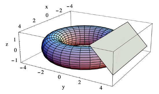
Example \(\PageIndex{2}\)

Let \(T\) be the torus parametrized by

\[ f(s, t)=((3+\cos (t)) \cos (s),(3+\cos (t)) \sin (s), \sin (t)) \nonumber \]

for \(0 \leq s \leq 2 \pi\) and \(0 \leq t \leq 2 \pi\). Then

\[ D f(s, t)=\left[\begin{array}{cc}
-(3+\cos (t)) \sin (s) & -\sin (t) \cos (s) \\
(3+\cos (t)) \cos (s) & -\sin (t) \sin (s) \\
0 & \cos (t)
\end{array}\right] . \nonumber \]

Thus, for example,

\[ \operatorname{Df}\left(\frac{\pi}{2}, \frac{\pi}{4}\right)=\left[\begin{array}{cc}
-\left(3+\frac{1}{\sqrt{2}}\right) & 0 \\
0 & -\frac{1}{\sqrt{2}} \\
0 & \frac{1}{\sqrt{2}}
\end{array}\right] . \nonumber \]

Since

\[ f\left(\frac{\pi}{2}, \frac{\pi}{4}\right)=\left(0,3+\frac{1}{\sqrt{2}}, \frac{1}{\sqrt{2}}\right) \text {, } \nonumber \]

the best affine approximation to \(f\) at \(\left(\frac{\pi}{2}, \frac{\pi}{4}\right)\) is

\[ A(s, t)=\left[\begin{array}{cc}
-\left(3+\frac{1}{\sqrt{2}}\right) & 0 \\
0 & -\frac{1}{\sqrt{2}} \\
0 & \frac{1}{\sqrt{2}}
\end{array}\right]\left[\begin{array}{c}
s-\frac{\pi}{2} \\
t-\frac{\pi}{4}
\end{array}\right]+\left[\begin{array}{c}
0 \\
3+\frac{1}{\sqrt{2}} \\
\frac{1}{\sqrt{2}}
\end{array}\right] \nonumber \]

\[ =\left[\begin{array}{c}
-\left(3+\frac{1}{\sqrt{2}}\right) \\
0 \\
0
\end{array}\right]\left(s-\frac{\pi}{2}\right)+\left[\begin{array}{c}
0 \\
-\frac{1}{\sqrt{2}} \\
\frac{1}{\sqrt{2}}
\end{array}\right]\left(t-\frac{\pi}{4}\right)+\left[\begin{array}{c}
0 \\
3+\frac{1}{\sqrt{2}} \\
\frac{1}{\sqrt{2}}
\end{array}\right] . \nonumber \]

Hence

\[ \begin{aligned}
&x=-\left(3+\frac{1}{\sqrt{2}}\right)\left(s-\frac{\pi}{2}\right), \\
&y=-\frac{1}{\sqrt{2}}\left(t-\frac{\pi}{4}\right)+3+\frac{1}{\sqrt{2}}, \\
&z=\frac{1}{\sqrt{2}}\left(t-\frac{\pi}{4}\right)+\frac{1}{\sqrt{2}},
\end{aligned} \]

are parametric equations for the plane \(P\) tangent to \(T\) at \(\left(0,3+\frac{1}{\sqrt{2}}, \frac{1}{\sqrt{2}}\right)\). See Figure 4.2.1.

Figure \(\PageIndex{1}\): Torus with a tangent plane

Chain rule

We are now in a position to state the chain rule in its most general form. Consider functions \(g: \mathbb{R}^{m} \rightarrow \mathbb{R}^{q}\) and \(f: \mathbb{R}^{q} \rightarrow \mathbb{R}^{n}\) and suppose \(g\) is differentiable at \(\mathbf{c}\) and \(f\) is differentiable at \(g(\mathbf{c})\). Let \(h: \mathbb{R}^{m} \rightarrow \mathbb{R}^{n}\) be the composition \(h(\mathbf{x})=f(g(\mathbf{x}))\) and denote the coordinate functions of \(f\), \(g\), and \(h\) by \(f_{i}, i=1,2, \ldots, n, g_{j}, j=1,2 \ldots, q\), and \(h_{k}, k=1,2, \ldots, n\), respectively. Then, for \(k=1,2, \ldots, n\),

\[ h_{k}\left(x_{1}, x_{2}, \ldots, x_{m}\right)=f_{k}\left(g_{1}\left(x_{1}, x_{2}, \ldots, x_{m}\right), g_{2}\left(x_{1}, x_{2}, \ldots, x_{m}\right), \ldots, g_{q}\left(x_{1}, x_{2}, \ldots, x_{m}\right)\right) . \nonumber \]

Now if we fix \(m-1\) of the variables \(x_{1}, x_{2}, \ldots, x_{m}\), say, all but \(x_j\), then \(h_k\) is the composition of a function from \(\mathbb{R}\) to \(\mathbb{R}^q\) with a function from \(\mathbb{R}^q\) to \(\mathbb{R}\). Thus we may use the chain rule from Section 3.3 to compute \(\frac{\partial}{\partial x_{j}} h_{k}(\mathbf{c})\), namely,

\[ \begin{gather}
\frac{\partial}{\partial x_{j}} h_{k}(\mathbf{c})=\nabla f_{k}(g(\mathbf{c})) \cdot\left(\frac{\partial}{\partial x_{j}} g_{1}(\mathbf{c}), \frac{\partial}{\partial x_{j}} g_{2}(\mathbf{c}), \ldots, \frac{\partial}{x_{j}} g_{q}(\mathbf{c})\right) \nonumber \\
=\frac{\partial}{\partial x_{1}} f_{k}(g(\mathbf{c})) \frac{\partial}{\partial x_{j}} g_{1}(\mathbf{c})+\frac{\partial}{\partial x_{2}} f_{k}(g(\mathbf{c})) \frac{\partial}{\partial x_{j}} g_{2}(\mathbf{c})+ \label{4.2.13} \\
\cdots+\frac{\partial}{\partial x_{q}} f_{k}(g(\mathbf{c})) \frac{\partial}{\partial x_{j}} g_{q}(\mathbf{c}). \nonumber
\end{gather} \]

Hence \(\frac{\partial}{\partial x_{j}} h_{k}(\mathbf{c})\) is equal to the dot product of the \(k\)th row of \(D f(g(\mathbf{c}))\) with the \(j\)th column of \(D g(\mathbf{c})\). Moreover, if \(g\) is \(C^1\) on an open ball about \(\mathbf{c}\) and \(f\) is \(C^1\) on an open ball about \(g(\mathbf{c})\), then (\(\ref{4.2.13}\)) shows that \(\frac{\partial}{\partial x_{j}} h_{k}\) is continuous on an open ball about \(\mathbf{c}\). It follows from our results in Section 3.3 that \(h\) is differentiable at \(\mathbf{c}\). Since \(\frac{\partial}{\partial x_{j}} h_{k}\) is the entry in the \(k\)th row and \(j\)th column of \(\operatorname{Dh}(\mathbf{c})\), (\(\ref{4.2.13}\)) implies \(\operatorname{Dh}(\mathbf{c})=D f(g(\mathbf{c})) D g(\mathbf{c})\). This result, the chain rule, may be proven without assuming that \(f\) and \(g\) are both \(C^1\), and so we state the more general result in the following theorem.

Theorem: Chain Rule \(\PageIndex{3}\)

If \(g: \mathbb{R}^{m} \rightarrow \mathbb{R}^{q}\) is differentiable at \(\mathbf{c}\) and \(f: \mathbb{R}^{q} \rightarrow \mathbb{R}^{n}\) is differentiable at \(g(\mathbf{c})\), then \(f \circ g\) is differentiable at \(\mathbf{c}\) and

\[ D(f \circ g)(\mathbf{c})=D f(g(\mathbf{c})) D g(\mathbf{c}) . \]

Equivalently, the chain rule says that if \(A\) is the best affine approximation to \(g\) at \(\mathbf{c}\) and \(B\) is the best affine approximation to \(f\) at \(g(\mathbf{c})\), then \(B \circ A\) is the best affine approximation to \(f \circ g\) at \(\mathbf{c}\). That is, the best affine approximation to a composition of functions is the composition of the individual best affine approximations.

Example \(\PageIndex{3}\)

Suppose \(g: \mathbb{R}^{2} \rightarrow \mathbb{R}^{3}\) is defined by

\[ g(s, t)=(\cos (s) \sin (t), \sin (s) \sin (t), \cos (t)) \nonumber \]

and \(f: \mathbb{R}^{3} \rightarrow \mathbb{R}^{2}\) is defined by

\[ f(x, y, z)=\left(10 x y z, x^{2}-y z\right) . \nonumber \]

Then

\[ D g(s, t)=\left[\begin{array}{cc}
-\sin (s) \sin (t) & \cos (s) \cos (t) \\
\cos (s) \sin (t) & \sin (s) \cos (t) \\
0 & -\sin (t)
\end{array}\right] \nonumber \]

and

\[ D f(x, y, z)=\left[\begin{array}{ccc}
10 y z & 10 x z & 10 x y \\
2 x & -z & -y
\end{array}\right] . \nonumber \]

Let \(h(s, t)=f(g(s, t))\). To find \(D h\left(\frac{\pi}{4}, \frac{\pi}{4}\right)\), we first note that

\[ g\left(\frac{\pi}{4}, \frac{\pi}{4}\right)=\left(\frac{1}{2}, \frac{1}{2}, \frac{1}{\sqrt{2}}\right) , \nonumber \]

\[ D g\left(\frac{\pi}{4}, \frac{\pi}{4}\right)=\left[\begin{array}{rr}
-\frac{1}{2} & \frac{1}{2} \\
\frac{1}{2} & \frac{1}{2} \\
0 & -\frac{1}{\sqrt{2}}
\end{array}\right] \nonumber \]

and

\[ D f\left(g\left(\frac{\pi}{4}, \frac{\pi}{4}\right)\right)=D f\left(\frac{1}{2}, \frac{1}{2}, \frac{1}{\sqrt{2}}\right)=\left[\begin{array}{ccc}
\frac{5}{\sqrt{2}} & \frac{5}{\sqrt{2}} & \frac{5}{2} \\
1 & -\frac{1}{\sqrt{2}} & -\frac{1}{2}
\end{array}\right] . \nonumber \]

Thus

\[ \begin{aligned}
\operatorname{Dh}\left(\frac{\pi}{4}, \frac{\pi}{4}\right) &=D f\left(g\left(\frac{\pi}{4}, \frac{\pi}{4}\right)\right) D g\left(\frac{\pi}{4}, \frac{\pi}{4}\right) \\
&=\left[\begin{array}{ccc}
\frac{5}{\sqrt{2}} & \frac{5}{\sqrt{2}} & \frac{5}{2} \\
1 & -\frac{1}{\sqrt{2}} & -\frac{1}{2}
\end{array}\right]\left[\begin{array}{rr}
-\frac{1}{2} & \frac{1}{2} \\
\frac{1}{2} & \frac{1}{2} \\
0 & -\frac{1}{\sqrt{2}}
\end{array}\right] \\
&=\left[\begin{array}{cc}
0 & \frac{5}{2 \sqrt{2}} \\
-\frac{1+\sqrt{2}}{2 \sqrt{2}} & \frac{1}{2}
\end{array}\right] .
\end{aligned} \]