4.4: Green's Theorem

Green’s theorem is an example from a family of theorems which connect line integrals (and their higher-dimensional analogues) with the definite integrals we studied in Section 3.6. We will first look at Green’s theorem for rectangles, and then generalize to more complex curves and regions in \(\mathbb{R}^2\).

Green’s theorem for rectangles

Suppose \(F: \mathbb{R}^{2} \rightarrow \mathbb{R}^{2}\) is \(C^1\) on an open set containing the closed rectangle

\[ D=[a, b] \times[c, d] , \nonumber \]

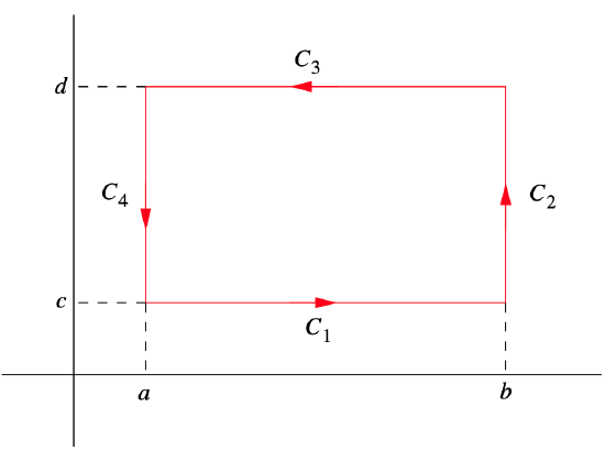
and let \(F_1\) and \(F_2\) be the coordinate functions of \(F\). If \(C\) denotes the boundary of \(D\), oriented in the clockwise direction, then we may decompose \(C\) into the four curves \(C_1\), \(C_2\), \(C_3\), and \(C_4\) shown in Figure 4.4.1.

Figure \(\PageIndex{1}\): The boundary of a rectangle decomposed into four smooth curves

Then

\[ \alpha(t)=(t, c) , \nonumber \]

\(a \leq t \leq b\), is a smooth parametrization of \(C_1\),

\[ \beta(t)=(b, t) , \nonumber \]

\(c \leq t \leq d\), is a smooth parametrization of \(C_2\),

\[ \gamma(t)=(t, d) , \nonumber \]

\(a \leq t \leq b\), is a smooth parametrization of \(-C_3\), and

\[ \delta(t)=(a, t) , \nonumber \]

\(c \leq t \leq d\), is a smooth parametrization of \(-C_4\). Now

\[ \begin{align}
\int_{C} F \cdot d s &=\int_{C_{1}} F \cdot d s+\int_{C_{2}} F \cdot d s+\int_{C_{3}} F \cdot d s+\int_{C_{4}} F \cdot d s \nonumber \\
&=\int_{C_{1}} F \cdot d s+\int_{C_{2}} F \cdot d s-\int_{-C_{3}} F \cdot d s-\int_{-C_{4}} F \cdot d s \label{4.4.1}
\end{align} \]

and

\[ \int_{C_{1}} F \cdot d s=\int_{a}^{b}\left(\left(F_{1}(t, c), F_{2}(t, c)\right) \cdot(1,0) d t=\int_{a}^{b} F_{1}(t, c) d t,\right. , \label{4.4.2} \]

\[ \int_{C_{2}} F \cdot d s=\int_{c}^{d}\left(\left(F_{1}(b, t), F_{2}(b, t)\right) \cdot(0,1) d t=\int_{c}^{c} F_{2}(b, t) d t\right. , \label{4.4.3} \]

\[ \int_{-C_{3}} F \cdot d s=\int_{a}^{b}\left(\left(F_{1}(t, d), F_{2}(t, d)\right) \cdot(1,0) d t=\int_{a}^{b} F_{1}(t, d) d t\right. , \label{4.4.4} \]

and

\[ \int_{-C_{4}} F \cdot d s=\int_{c}^{d}\left(\left(F_{1}(a, t), F_{2}(a, t)\right) \cdot(0,1) d t=\int_{c}^{c} F_{2}(a, t) d t\right. , \label{4.4.5} \]

Hence, inserting (\(\ref{4.4.2}\)) through (\(\ref{4.4.5}\)) into (\(\ref{4.4.1}\)),

\[ \begin{align}
\int_{C} F \cdot d s &=\int_{a}^{b} F_{1}(t, c) d t+\int_{c}^{d} F_{2}(b, t) d t-\int_{a}^{b} F_{1}(t, d) d t-\int_{c}^{d} F_{2}(a, t) d t \nonumber \\
&=\int_{c}^{d}\left(F_{2}(b, t)-F_{2}(a, t)\right) d t-\int_{a}^{b}\left(F_{1}(t, d)-F_{1}(t, c)\right) d t . \label{4.4.6}
\end{align} \]

Now, by the Fundamental Theorem of Calculus, for a fixed value of \(t\),

\[ \int_{a}^{b} \frac{\partial}{\partial x} F_{2}(x, t) d x=F_{2}(b, t)-F_{2}(a, t) \label{4.4.7} \]

and

\[ \int_{c}^{d} \frac{\partial}{\partial y} F_{1}(t, y) d y=F_{1}(t, d)-F_{1}(t, c) . \label{4.4.8} \]

Thus, combining (\(\ref{4.4.7}\)) and (\(\ref{4.4.8}\)) with (\(\ref{4.4.6}\)), we have

\[ \begin{align}
\int_{C} F \cdot d s &=\int_{c}^{d} \int_{a}^{b} \frac{\partial}{\partial x} F_{2}(x, t) d x d t-\int_{a}^{b} \int_{c}^{d} \frac{\partial}{\partial y} F_{1}(t, y) d y d t \nonumber \\
&=\int_{c}^{d} \int_{a}^{b} \frac{\partial}{\partial x} F_{2}(x, y) d x d y-\int_{a}^{b} \int_{c}^{d} \frac{\partial}{\partial y} F_{1}(x, y) d y d x \nonumber \\
&=\int_{c}^{d} \int_{a}^{b}\left(\frac{\partial}{\partial x} F_{2}(x, y)-\frac{\partial}{\partial y} F_{1}(x, y)\right) d x d y \label{4.4.9}
\end{align} \]

If we let \(p=F_{1}(x, y), q=F_{2}(x, y)\), and \(\partial D=C\) (a common notation for the boundary of \(D\)), then we may rewrite (\(\ref{4.4.9}\)) as

\[ \int_{\partial D} p d x+q d y=\iint_{D}\left(\frac{\partial q}{\partial x}-\frac{\partial p}{\partial y}\right) d x d y . \]

This is Green’s theorem for a rectangle.

Example \(\PageIndex{1}\)

If \(D=[1,3] \times[2,5]\), then

\[ \begin{aligned}
\int_{\partial D} x y d x+x d y &=\iint_{D}\left(\frac{\partial}{\partial x} x-\frac{\partial}{\partial y} x y\right) d x d y \\
&=\int_{1}^{3} \int_{2}^{5}(1-x) d y d x \\
&=\int_{1}^{3} 3(1-x) d x \\
&=\left.3 x\right|_{1} ^{3}-\left.\frac{3}{2} x^{2}\right|_{1} ^{3} \\
&=-6 .
\end{aligned} \]

Clearly, this is simpler than evaluating the line integral directly.

Green’s theorem for regions of Type III

Green’s theorem holds for more general regions than rectangles. We will confine ourselves here to discussing regions known as regions of Type III, but it is not hard to generalize to regions which may be subdivided into regions of this type (for an example, see Problem 12). Recall from Section 3.6 that we say a region \(D\) in \(\mathbb{R}^2\) is of Type I if there exist real numbers \(a<b\) and continuous functions \(\alpha: \mathbb{R} \rightarrow \mathbb{R}\) and \(\beta: \mathbb{R} \rightarrow \mathbb{R}\) such that

\[ D=\{(x, y): a \leq x \leq b, \alpha(x) \leq y \leq \beta(x)\} . \]

We say a region \(D\) in \(\mathbb{R}^2\) is of Type II if there exist real numbers \(c\) and \(d\) and continuous functions \(\gamma: \mathbb{R} \rightarrow \mathbb{R}\) and \(\delta: \mathbb{R} \rightarrow \mathbb{R}\) such that

\[ D=\{(x, y): c \leq y \leq d, \gamma(y) \leq x \leq \delta(y)\} . \]

Definition \(\PageIndex{1}\)

We call a region \(D\) in \(\mathbb{R}^2\) which is both of Type I and of Type II a region of Type III.

Example \(\PageIndex{2}\)

In Section 3.6, we saw that the triangle \(T\) with vertices at (0,0), (1,0), and (1,1) and the closed disk

\[ D=\bar{B}^{2}((0,0), 1)=\left\{(x, y): x^{2}+y^{2} \leq 1\right\} \nonumber \]

are of both Type I and Type II. Thus \(T\) and \(D\) are regions of Type III. We also saw that the region \(E\) beneath the graph of \(y=x^2\) and above the interval [−1,1] is of Type I, but not of Type II. Hence \(E\) is not of Type III.

Example \(\PageIndex{3}\)

Any closed rectangle in \(\mathbb{R}^2\) is a region of Type III, as is any closed region bounded by an ellipse.

Now suppose \(D\) is a region of Type III and \(\partial D\) is the boundary of \(D\), that is, the curve enclosing \(D\), oriented counterclockwise. Let \(F: \mathbb{R}^{2} \rightarrow \mathbb{R}^{2}\) be a \(C^1\) vector field, with coordinate functions \(p=F_{1}(x, y)\) and \(q=F_{2}(x, y)\). We will first prove that

\[ \int_{\partial D} p d x=-\iint_{D} \frac{\partial p}{\partial y} d x d y . \]

Since \(D\) is, in particular, a region of Type I, there exist continuous functions \(\alpha\) and \(\beta\) such that

\[ D=\{(x, y): a \leq x \leq b, \alpha(x) \leq y \leq \beta(x)\} . \]

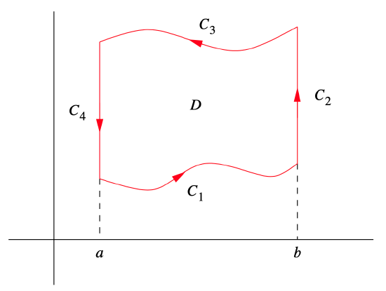
In addition, we will assume that \(\alpha\) and \(\beta\) are both differentiable (without this assumption the line integral of \(F\) along \(\partial D\) would not be defined). As with the rectangle in the previous proof, we may decompose \(\partial D\) into four curves, \(C_1\), \(C_2\), \(C_3\), and \(C_4\), as shown in Figure 4.4.2.

Figure \(\PageIndex{2}\): Decomposing the boundary of a region of Type I

Then

\[ \varphi_{1}(t)=(t, \alpha(t)) , \nonumber \]

\(a \leq t \leq b\), is a smooth parametrization of \(C_1\),

\[ \varphi_{2}(t)=(b, t) , \nonumber \]

\(\alpha(b) \leq t \leq \beta(b)\), is a smooth parametrization of \(C_2\),

\[ \varphi_{3}(t)=(t, \beta(t)) , \nonumber \]

\(a \leq t \leq b\), is a smooth parametrization of \(-C_3\), and

\[ \varphi_{4}(t)=(a, t) , \nonumber \]

\(\alpha(a) \leq t \leq \beta(a)\), is a smooth parametrization of \(-C_4\). Now

\[ \int_{\partial D} p d x=\int_{C_{1}} p d x+\int_{C_{2}} p d x-\int_{-C_{3}} p d x-\int_{-C_{4}} p d x ,\]

where

\[ \int_{C_{1}} p d x=\int_{a}^{b}\left(F_{1}(t, \alpha(t)), 0\right) \cdot\left(1, \alpha^{\prime}(t)\right) d t=\int_{a}^{b} F_{1}(t, \alpha(t)) d t, \]

\[ \int_{C_{2}} p d x=\int_{\alpha(b)}^{\beta(b)}\left(F_{1}(b, t), 0\right) \cdot(0,1) d t=\int_{\alpha(b)}^{\beta(b)} 0 d t=0 ,\]

\[ \int_{-C_{3}} p d x=\int_{a}^{b}\left(F_{1}(t, \beta(t)), 0\right) \cdot\left(1, \beta^{\prime}(t)\right) d t=\int_{a}^{b} F_{1}(t, \beta(t)) d t , \]

and

\[ \int_{-C_{4}} p d x=\int_{\alpha(a)}^{\beta(a)}\left(F_{1}(a, t), 0\right) \cdot(0,1) d t=\int_{\alpha(a)}^{\beta(a)} 0 d t=0 .\]

Hence

\[ \begin{align}
\int_{\partial D} p d x &=\int_{a}^{b} F_{1}(t, \alpha(t)) d t-\int_{a}^{b} F_{1}(t, \beta(t)) d t \nonumber \\
&=-\int_{a}^{b}\left(F_{1}(t, \beta(t))-F_{1}(t, \alpha(t))\right) d t \label{4.4.20}
\end{align} \]

Now, by the Fundamental Theorem of Calculus,

\[ \int_{\alpha(t)}^{\beta(t)} \frac{\partial}{\partial y} F_{1}(t, y) d y=F_{1}(t, \beta(t))-F_{1}(t, \alpha(t)) , \]

and so

\[ \begin{align}
\int_{\partial D} p d x &=-\int_{a}^{b} \int_{\alpha(t)}^{\beta(t)} \frac{\partial}{\partial y} F_{1}(t, y) d y d t \nonumber \\
&=-\int_{a}^{b} \int_{\alpha(x)}^{\beta(x)} \frac{\partial}{\partial y} F_{1}(x, y) d y d x \nonumber \\
&=-\iint_{D} \frac{\partial p}{\partial y} d x d y . \label{4.4.22}
\end{align} \]

A similar calculation, treating \(D\) as a region of Type II, shows that

\[ \int_{\partial D} q d y=\iint_{D} \frac{\partial q}{\partial x} d x d y . \label{4.4.23} \]

(You are asked to verify this in Exercise 7.) Putting (\(\ref{4.4.22}\)) and (\(\ref{4.4.23}\)) together, we have

\[ \begin{align}
\int_{\partial D} F \cdot d s=\int_{\partial D} p d x+q d y &=-\iint_{D} \frac{\partial p}{\partial y} d x d y+\iint_{D} \frac{\partial q}{\partial x} d x d y \nonumber \\
&=\iint_{D}\left(\frac{\partial q}{\partial x}-\frac{\partial p}{\partial y}\right) d x d y \label{4.4.24}
\end{align} \]

Green's Theorem \(\PageIndex{1}\)

Suppose \(D\) is a region of Type III, \(\partial D\) is the boundary of \(D\) with counterclockwise orientation, and the curves describing \(\partial D\) are differentiable. Let \(F: \mathbb{R}^{2} \rightarrow \mathbb{R}^{2} \) be a \(C^1\) vector field, with coordinate functions \(p=F_{1}(x, y)\) and \(q=F_{2}(x, y)\). Then

\[ \int_{\partial D} p d x+q d y=\iint_{D}\left(\frac{\partial q}{\partial x}-\frac{\partial p}{\partial y}\right) d x d y . \]

Example \(\PageIndex{4}\)

Let \(D\) be the region bounded by the triangle with vertices at (0,0), (2,0), and (0,3), as shown in Figure 4.4.3.

Figure \(\PageIndex{3}\): A triangle with counterclockwise orientation

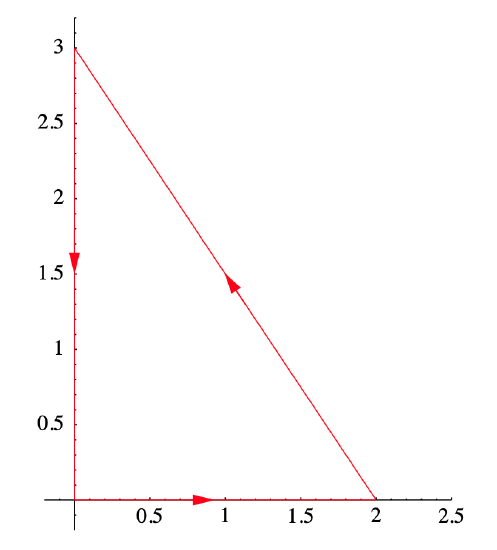
If we orient \(\partial D\) in the counterclockwise direction, then

\[ \begin{aligned}
\int_{\partial D}\left(3 x^{2}+y\right) d x+5 x d y &=\iint_{D}\left(\frac{\partial}{\partial x}(5 x)-\frac{\partial}{\partial y}\left(3 x^{2}+y\right)\right) d x d y \\
&=\iint_{D}(5-1) d x d y \\
&=4 \iint_{D} d x d y \\
&=(4)(3) \\
&=12,
\end{aligned} \]

where we have used the fact that the area of \(D\) is 3 to evaluate the double integral.

The line integral in the previous example reduced to finding the area of the region \(D\). This can be exploited in the reverse direction to compute the area of a region. For example, given a region \(D\) with area \(A\) and boundary \(\partial D\), it follows from Green’s theorem that

\[ A=\iint_{D} d x d y=\int_{\partial D} p d x+q d y \]

for any choice of \(p\) and \(q\) which have the property that

\[ \frac{\partial q}{\partial x}-\frac{\partial p}{\partial y}=1 . \]

For example, letting \(p = 0\) and \(q = x\), we have

\[ A=\int_{\partial D} x d y \label{4.4.28} \]

and, letting \(p = −y\) and \(q = 0\), we have

\[ A=-\int_{\partial D} y d x . \label{4.4.29} \]

The next example illustrates using the average of (\(\ref{4.4.28}\)) and (\(\ref{4.4.29}\)) to find \(A\):

\[ A=\frac{1}{2}\left(\int_{\partial D} x d y-\int_{\partial D} y d x\right)=\frac{1}{2} \int_{\partial D} x d y-y d x . \]

Example \(\PageIndex{5}\)

Let \(A\) be the area of the region \(D\) bounded by the ellipse with equation

\[ \frac{x^{2}}{a^{2}}+\frac{y^{2}}{b^{2}}=1 , \nonumber \]

where \(a > 0\) and \(b>0\), as shown in Figure 4.4.4.

Figure 4.4.4 The ellipse \(\frac{x^{2}}{a^{2}}+\frac{y^{2}}{b^{2}}=1\) with counterclockwise orientation

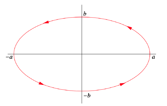
Since we may parametrize \(\partial D\), with counterclockwise orientation, by

\[ \varphi(t)=(a \cos (t), b \sin (t)) , \nonumber \]

\(0 \leq t \leq 2 \pi\), we have

\[ \begin{aligned}
A &=\frac{1}{2} \int_{\partial D} x d y-y d x \\
&=\frac{1}{2} \int_{0}^{2 \pi}(-b \sin (t), a \cos (t)) \cdot(-a \sin (t), b \cos (t) d t\\
&=\frac{1}{2} \int_{0}^{2 \pi}\left(a b \sin ^{2}(t)+a b \cos ^{2}(t)\right) d t \\
&=\frac{a b}{2} \int_{0}^{2 \pi} d t \\
&=\left(\frac{a b}{2}\right)(2 \pi) \\
&=\pi a b.
\end{aligned} \]