Mathematics LibreTexts

4.4.E: Green's Theorem (Exercises)

  • Page ID
    78232
  • \( \newcommand{\vecs}[1]{\overset { \scriptstyle \rightharpoonup} {\mathbf{#1}} } \)

    \( \newcommand{\vecd}[1]{\overset{-\!-\!\rightharpoonup}{\vphantom{a}\smash {#1}}} \)

    \( \newcommand{\id}{\mathrm{id}}\) \( \newcommand{\Span}{\mathrm{span}}\)

    ( \newcommand{\kernel}{\mathrm{null}\,}\) \( \newcommand{\range}{\mathrm{range}\,}\)

    \( \newcommand{\RealPart}{\mathrm{Re}}\) \( \newcommand{\ImaginaryPart}{\mathrm{Im}}\)

    \( \newcommand{\Argument}{\mathrm{Arg}}\) \( \newcommand{\norm}[1]{\| #1 \|}\)

    \( \newcommand{\inner}[2]{\langle #1, #2 \rangle}\)

    \( \newcommand{\Span}{\mathrm{span}}\)

    \( \newcommand{\id}{\mathrm{id}}\)

    \( \newcommand{\Span}{\mathrm{span}}\)

    \( \newcommand{\kernel}{\mathrm{null}\,}\)

    \( \newcommand{\range}{\mathrm{range}\,}\)

    \( \newcommand{\RealPart}{\mathrm{Re}}\)

    \( \newcommand{\ImaginaryPart}{\mathrm{Im}}\)

    \( \newcommand{\Argument}{\mathrm{Arg}}\)

    \( \newcommand{\norm}[1]{\| #1 \|}\)

    \( \newcommand{\inner}[2]{\langle #1, #2 \rangle}\)

    \( \newcommand{\Span}{\mathrm{span}}\) \( \newcommand{\AA}{\unicode[.8,0]{x212B}}\)

    \( \newcommand{\vectorA}[1]{\vec{#1}}      % arrow\)

    \( \newcommand{\vectorAt}[1]{\vec{\text{#1}}}      % arrow\)

    \( \newcommand{\vectorB}[1]{\overset { \scriptstyle \rightharpoonup} {\mathbf{#1}} } \)

    \( \newcommand{\vectorC}[1]{\textbf{#1}} \)

    \( \newcommand{\vectorD}[1]{\overrightarrow{#1}} \)

    \( \newcommand{\vectorDt}[1]{\overrightarrow{\text{#1}}} \)

    \( \newcommand{\vectE}[1]{\overset{-\!-\!\rightharpoonup}{\vphantom{a}\smash{\mathbf {#1}}}} \)

    \( \newcommand{\vecs}[1]{\overset { \scriptstyle \rightharpoonup} {\mathbf{#1}} } \)

    \( \newcommand{\vecd}[1]{\overset{-\!-\!\rightharpoonup}{\vphantom{a}\smash {#1}}} \)

    \(\newcommand{\avec}{\mathbf a}\) \(\newcommand{\bvec}{\mathbf b}\) \(\newcommand{\cvec}{\mathbf c}\) \(\newcommand{\dvec}{\mathbf d}\) \(\newcommand{\dtil}{\widetilde{\mathbf d}}\) \(\newcommand{\evec}{\mathbf e}\) \(\newcommand{\fvec}{\mathbf f}\) \(\newcommand{\nvec}{\mathbf n}\) \(\newcommand{\pvec}{\mathbf p}\) \(\newcommand{\qvec}{\mathbf q}\) \(\newcommand{\svec}{\mathbf s}\) \(\newcommand{\tvec}{\mathbf t}\) \(\newcommand{\uvec}{\mathbf u}\) \(\newcommand{\vvec}{\mathbf v}\) \(\newcommand{\wvec}{\mathbf w}\) \(\newcommand{\xvec}{\mathbf x}\) \(\newcommand{\yvec}{\mathbf y}\) \(\newcommand{\zvec}{\mathbf z}\) \(\newcommand{\rvec}{\mathbf r}\) \(\newcommand{\mvec}{\mathbf m}\) \(\newcommand{\zerovec}{\mathbf 0}\) \(\newcommand{\onevec}{\mathbf 1}\) \(\newcommand{\real}{\mathbb R}\) \(\newcommand{\twovec}[2]{\left[\begin{array}{r}#1 \\ #2 \end{array}\right]}\) \(\newcommand{\ctwovec}[2]{\left[\begin{array}{c}#1 \\ #2 \end{array}\right]}\) \(\newcommand{\threevec}[3]{\left[\begin{array}{r}#1 \\ #2 \\ #3 \end{array}\right]}\) \(\newcommand{\cthreevec}[3]{\left[\begin{array}{c}#1 \\ #2 \\ #3 \end{array}\right]}\) \(\newcommand{\fourvec}[4]{\left[\begin{array}{r}#1 \\ #2 \\ #3 \\ #4 \end{array}\right]}\) \(\newcommand{\cfourvec}[4]{\left[\begin{array}{c}#1 \\ #2 \\ #3 \\ #4 \end{array}\right]}\) \(\newcommand{\fivevec}[5]{\left[\begin{array}{r}#1 \\ #2 \\ #3 \\ #4 \\ #5 \\ \end{array}\right]}\) \(\newcommand{\cfivevec}[5]{\left[\begin{array}{c}#1 \\ #2 \\ #3 \\ #4 \\ #5 \\ \end{array}\right]}\) \(\newcommand{\mattwo}[4]{\left[\begin{array}{rr}#1 \amp #2 \\ #3 \amp #4 \\ \end{array}\right]}\) \(\newcommand{\laspan}[1]{\text{Span}\{#1\}}\) \(\newcommand{\bcal}{\cal B}\) \(\newcommand{\ccal}{\cal C}\) \(\newcommand{\scal}{\cal S}\) \(\newcommand{\wcal}{\cal W}\) \(\newcommand{\ecal}{\cal E}\) \(\newcommand{\coords}[2]{\left\{#1\right\}_{#2}}\) \(\newcommand{\gray}[1]{\color{gray}{#1}}\) \(\newcommand{\lgray}[1]{\color{lightgray}{#1}}\) \(\newcommand{\rank}{\operatorname{rank}}\) \(\newcommand{\row}{\text{Row}}\) \(\newcommand{\col}{\text{Col}}\) \(\renewcommand{\row}{\text{Row}}\) \(\newcommand{\nul}{\text{Nul}}\) \(\newcommand{\var}{\text{Var}}\) \(\newcommand{\corr}{\text{corr}}\) \(\newcommand{\len}[1]{\left|#1\right|}\) \(\newcommand{\bbar}{\overline{\bvec}}\) \(\newcommand{\bhat}{\widehat{\bvec}}\) \(\newcommand{\bperp}{\bvec^\perp}\) \(\newcommand{\xhat}{\widehat{\xvec}}\) \(\newcommand{\vhat}{\widehat{\vvec}}\) \(\newcommand{\uhat}{\widehat{\uvec}}\) \(\newcommand{\what}{\widehat{\wvec}}\) \(\newcommand{\Sighat}{\widehat{\Sigma}}\) \(\newcommand{\lt}{<}\) \(\newcommand{\gt}{>}\) \(\newcommand{\amp}{&}\) \(\definecolor{fillinmathshade}{gray}{0.9}\)

    Exercise \(\PageIndex{1}\)

    Let \(D\) be the closed rectangle in \(\mathbb{R}^2\) with vertices at (0,0), (2,0), (2,4), and (0,4), with boundary \(\partial D\) oriented counterclockwise. Use Green’s theorem to evaluate the following line integrals.

    (a) \(\int_{\partial D} 2 x y d x+3 x^{2} d y\)

    (b) \(\int_{\partial D} y d x+x d y\)

    Answer

    (a) \(\int_{\partial D} 2 x y d x+3 x^{2} d y=80\)

    Exercise \(\PageIndex{2}\)

    Let \(D\) be the triangle in \(\mathbb{R}^2\) with vertices at (0,0), (2,0), and (0,4), with boundary \(\partial D\) oriented counterclockwise. Use Green’s theorem to evaluate the following line integrals.

    (a) \(\int_{\partial D} 2 x y^{2} d x+4 x d y\)

    (b) \(\int_{\partial D} y d x+x d y\)

    (c) \(\int_{\partial D} y d x-x d y\)

    Answer

    (a) \(\int_{\partial D} 2 x y^{2} d x+4 x d y=\frac{16}{3} \text { (c) } \int_{\partial D} y d x-x d y=-8\)

    Exercise \(\PageIndex{3}\)

    Use Green’s theorem to find the area of a circle of radius \(r\).

    Exercise \(\PageIndex{4}\)

    Use Green’s theorem to find the area of the region \(D\) enclosed by the hypocycloid

    \[ x^{\frac{2}{3}}+y^{\frac{2}{3}}=a^{\frac{2}{3}} , \nonumber \]

    where \(a > 0\). Note that we may parametrize this curve using

    \[ \varphi(t)=\left(a \cos ^{3}(t), a \sin ^{3}(t)\right) , \nonumber \]

    \(0 \leq t \leq 2 \pi\).

    Answer

    \(\frac{3}{8} \pi a^{2}\)

    Exercise \(\PageIndex{5}\)

    Use Green’s theorem to find the area of the region enclosed by one “petal” of the curve parametrized by

    \[ \varphi(t)=(\sin (2 t) \cos (t), \sin (2 t) \sin (t)) . \nonumber \]

    Answer

    \(\frac{\pi}{8}\)

    Exercise \(\PageIndex{6}\)

    Find the area of the region enclosed by the cardioid parametrized by

    \[ \varphi(t)=((2+\cos (t)) \cos (t),(2+\cos (t)) \sin (t)) , \nonumber \]

    \(0 \leq t \leq 2 \pi\).

    Answer

    \(\frac{9 \pi}{2}\)

    Exercise \(\PageIndex{7}\)

    Verify (4.4.23), thus completing the proof of Green’s theorem.

    Exercise \(\PageIndex{8}\)

    Suppose the vector field \(F: \mathbb{R}^{2} \rightarrow \mathbb{R}^{2}\) with coordinate functions \(p=F_{1}(x, y)\) and \(q=F_{2}(x, y)\) is \(C^1\) on an open set containing the Type III region \(D\). Moreover, suppose \(F\) is the gradient of a scalar function \(f: \mathbb{R}^{2} \rightarrow \mathbb{R}\).

    (a) Show that

    \[ \frac{\partial q}{\partial x}-\frac{\partial p}{\partial y}=0 \nonumber \]

    for all points \((x,y)\) in \(D\).

    (b) Use Green’s theorem to show that

    \[ \int_{\partial D} p d x+q d y=0 , \nonumber \]

    where \(\partial D\) is the boundary of \(D\) with counterclockwise orientation.

    Exercise \(\PageIndex{9}\)

    How many ways do you know to calculate the area of a circle?

    Exercise \(\PageIndex{10}\)

    Who was George Green?

    Exercise \(\PageIndex{11}\)

    Explain how Green’s theorem is a generalization of the Fundamental Theorem of Integral Calculus.

    Exercise \(\PageIndex{12}\)

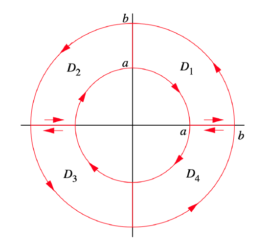
    Let \(b > a\), let \(C_1\) be the circle of radius \(b\) centered at the origin, and let \(C_2\) be the circle of radius \(a\) centered at the origin. If \(D\) is the annular region between \(C_1\) and \(C_2\) and \(F\) is a \(C^1\) vector field with coordinate functions \(p=F_{1}(x, y)\) and \(q=F_{2}(x, y)\), show that

    \[ \iint_{D}\left(\frac{\partial q}{\partial x}-\frac{\partial p}{\partial y}\right) d x d y=\int_{C_{1}} p d x+q d y+\int_{C_{2}} p d x+q d y , \nonumber \]

    where \(C_1\) is oriented in the counterclockwise direction and \(C_2\) is oriented in the clockwise direction. (Hint: Decompose \(D\) into Type III regions \(D_1\), \(D_2\), \(D_3\), and \(D_4\), each with boundary oriented counterclockwise, as shown in Figure 4.4.5.)

    Screen Shot 2021-08-24 at 08.37.28.png
    Figure \(\PageIndex{5}\): Decomposition of an annulus into regions of Type III


    This page titled 4.4.E: Green's Theorem (Exercises) is shared under a CC BY-NC-SA 1.0 license and was authored, remixed, and/or curated by Dan Sloughter via source content that was edited to the style and standards of the LibreTexts platform.