12.3: Dijkstra's Algorithm for Shortest Paths

Just as with graphs, it is useful to assign weights to the directed edges of a digraph. Specifically, in this section we consider a pair $(\textbf{G},w)$ where $\textbf{G}=(V,E)$ is a digraph and $w:E \rightarrow \mathbb{N}_0$ is a function assigning to each directed edge $(x,y)$ a non-negative weight $w(x,y)$. However, in this section, we interpret weight as distance so that $w(x,y)$ is now called the length of the edge $(x,y)$. If $P=(r=u_0,u_1,…,u_t=x)$ is a directed path from $r$ to $x$, then the length of the path $P$ is just the sum of the lengths of the edges in the path, $\sum_{i=0}^{t-1} w(u_iu_{i+1})$. The distance from $r$ to $x$ is then defined to be the minimum length of a directed path from $r$ to $x$. Our goal in this section is to solve the following natural problem, which has many applications:

Problem 12.13.

For each vertex $x$, find the distance from $r$ to $x$. Also, find a shortest path from $r$ to $x$.

12.3.1 Description of the Algorithm

To describe Dijkstra's algorithm in a compact manner, it is useful to extend the definition of the function $w$. We do this by setting $w(x,y)= \infty$ when $x \neq y$ and $(x,y)$ is not a directed edge of $\textbf{G}$. In this way, we will treat $\infty$ as if it were a number (although it is not!).

We are now prepared to describe Dijkstra's Algorithm.

Algorithm 12.14 Dijkstra's Algorithm

Let $n=|V|$. At Step $i$, where $1≤i≤n$, we will have determined:

1. A sequence $σ=(v_1,v_2,v3,…,v_i)$ of distinct vertices from $\textbf{G}$ with $r=v_1$. These vertices are called permanent vertices, while the remaining vertices will be called temporary vertices.
2. For each vertex $x∈V$, we will have determined a number $δ(x)$ and a path $P(x)$ from $r$ to $x$ of length $δ(x)$.

Initialization (Step 1)

Set $i=1$. Set $δ(r)=0$ and let $P(r)=(r)$ be the trivial one-point path. Also, set $σ=(r)$. For each $x≠r$, set $δ(x)=w(r,x)$ and $P(x)=(r,x)$. Let $x$ be a temporary vertex for which $δ(x)$ is minimum. Set $v_2=x$, and update $σ$ by appending $v_2$ to the end of it. Increment $i$.

Inductive Step (Step $i, i > 1$)

If $i<n$, then for each temporary $x$, let

$δ(x)=min\{δ(x),δ(v_i)+w(v_i,x)\}$.

If this assignment results in a reduction in the value of $δ(x)$, let $P(x)$ be the path obtained by adding $x$ to the end of $P(v_i)$.

Let $x$ be a temporary vertex for which $δ(x)$ is minimum. Set $v_{i+1}=x$, and update $σ$ by appending $v_{i+1}$ to it. Increment $i$.

12.3.2 Example of Dijkstra's Algorithm

Before establishing why Dijkstra's algorithm works, it may be helpful to see an example of how it works. To do this, consider the digraph $\textbf{G}$ shown in Figure 12.15. For visual clarity, we have chosen a digraph which is an oriented graph, i.e., for each distinct pair $x,y$ of vertices, the graph contains at most one of the two possible directed edges $(x,y)$ and $(y,x)$.

Figure 12.15. A digraph with edge lengths

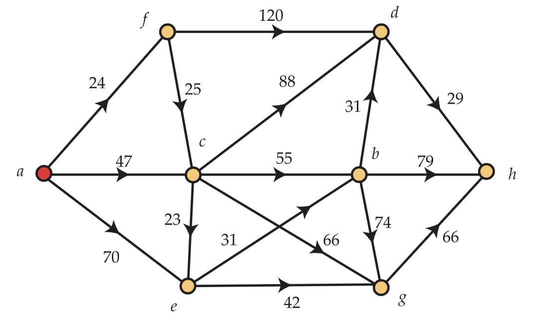
Suppose that the root vertex $r$ is the vertex labeled $a$. The initialization step of Dijkstra's algorithm then results in the following values for $δ$ and $P$:

Step 1. Initialization.

$σ=(a)$

$δ(a)=0;P(a)=(a)$

$δ(b)= \infty ;P(b)=(a,b)$

$δ(c)=47;P(c)=(a,c)$

$δ(d)= \infty ;P(d)=(a,d)$

$δ(e)=70;P(e)=(a,e)$

$δ(f)=24;P(f)=(a,f)$

$δ(g)= \infty ;P(g)=(a,g)$

$δ(h)= \infty ;P(h)=(a,h)$

Before finishing Step 1, the algorithm identifies vertex $f$ as closest to $a$ and appends it to $σ$, making $a$ permanent. When entering Step 2, Dijkstra's algorithm attempts to find shorter paths from $a$ to each of the temporary vertices by going through $f$. We call this process “scanning from vertex $f$.” In this scan, the path to vertex $d$ is updated, since $δ(f) + w(f,d) = 24 + 120 = 144 < \infty = w(a,d)$.

Step 2. Scan from vertex $f$.

$σ=(a,f)$

$δ(a)=0;P(a)=(a)$

$δ(b)= \infty;P(b)=(a,b)$

$δ(c)=47;P(c)=(a,c)$

$δ(d)=144=24+120=δ(f)+w(f,d);P(d)=(a,f,d)$ updated

$δ(e)=70;P(e)=(a,e)$

$δ(f)=24;P(f)=(a,f)$

$δ(g)= \infty ;P(g)=(a,f)$

$δ(h)= \infty ;P(h)=(a,h)$

Before proceeding to the next step, vertex $c$ is made permanent by making it $v_3$. In Step 3, therefore, the scan is from vertex $c$. Vertices $b, d$, and $g$ have their paths updated. However, although $δ(c)+w(c,e)=47+23=70=δ(e)$, we do not change $P(e)$ since $δ(e)$ is not decreased by routing $P(e)$ through $c$.

Step 3. Scan from vertex $c$.

$σ=(a,f,c)$

$δ(a)=0;P(a)=(a)$

$δ(b)=102=47+55=δ(c)+w(c,b);P(b)=(a,c,b)$ updated

$δ(c)=47;P(c)=(a,c)$

$δ(d)=135=47+88=δ(c)+w(c,d);P(d)=(a,c,d)$ updated

$δ(e)=70;P(e)=(a,e)$

$δ(f)=24;P(f)=(a,f)$

$δ(g)=113=47+66=δ(c)+w(c,g);P(g)=(a,c,g)$ updated

$δ(h)= \infty;P(h)=(a,h)$

Now vertex $e$ is made permanent.

Step 4. Scan from vertex e.

$σ=(a,f,c,e)$

$δ(a)=0;P(a)=(a)$

$δ(b)=101=70+31=δ(e)+w(e,b);P(b)=(a,e,b)$ updated

$δ(c)=47;P(c)=(a,c)$

$δ(d)=135;P(d)=(a,c,d)$

$δ(e)=70;P(e)=(a,e)$

$δ(f)=24;P(f)=(a,f)$

$δ(g)=112=70+42=δ(e)+w(e,g);P(g)=(a,e,g)$ updated

$δ(h)= \infty;P(h)=(a,h)$

Now vertex $b$ is made permanent.

Step 5. Scan from vertex b.

$σ=(a,f,c,e,b)$

$δ(a)=0;P(a)=(a)$

$δ(b)=101;P(b)=(a,e,b)$

$δ(c)=47;P(c)=(a,c)$

$δ(d)=132=101+31=δ(b)+w(b,d);P(d)=(a,e,b,d)$ updated

$δ(e)=70;P(e)=(a,e)$

$δ(f)=24;P(f)=(a,f)$

$δ(g)=112;P(g)=(a,e,g)$

$δ(h)=180=101+79=δ(b)+w(b,h);P(h)=(a,e,b,h)$ updated

Now vertex $g$ is made permanent.

Step 6. Scan from vertex g.

$σ=(a,f,c,e,b,g)$

$δ(a)=0;P(a)=(a)$

$δ(b)=101;P(b)=(a,e,b)$

$δ(c)=47;P(c)=(a,c)$

$δ(d)=132;P(d)=(a,e,b,d)$

$δ(e)=70;P(e)=(a,e)$

$δ(f)=24;P(f)=(a,f)$

$δ(g)=112;P(g)=(a,e,g)$

$δ(h)=178=112+66=δ(g)+w(g,h);P(h)=(a,e,g,h)$ updated

Now vertex $d$ is made permanent.

Step 7. Scan from vertex d.

$σ=(a,f,c,e,b,g,d)$

$δ(a)=0;P(a)=(a)$

$δ(b)=101;P(b)=(a,e,b)$

$δ(c)=47;P(c)=(a,c)$

$δ(d)=132;P(d)=(a,e,b,d)$

$δ(e)=70;P(e)=(a,e)$

$δ(f)=24;P(f)=(a,f)$

$δ(g)=112;P(g)=(a,e,g)$

$δ(h)=161=132+29=δ(d)+w(d,h);P(h)=(a,e,b,d,h)$ updated

Now vertex $h$ is made permanent. Since this is the last vertex, the algorithm halts and returns the following:

Final Results of Dijkstra's Algorithm.

$σ=(a,f,c,e,b,g,d,h)$

$δ(a)=0;P(a)=(a)$

$δ(b)=101;P(b)=(a,e,b)$

$δ(c)=47;P(c)=(a,c)$

$δ(d)=132;P(d)=(a,e,b,d)$

$δ(e)=70;P(e)=(a,e)$

$δ(f)=24;P(f)=(a,f)$

$δ(g)=112;P(g)=(a,e,g)$

$δ(h)=161;P(h)=(a,e,b,d,h)$

12.3.3 The Correctness of Dijkstra's Algorithm

Now that we've illustrated Dijkstra's algorithm, it's time to prove that it actually does what we claimed it does: find the distance from the root vertex to each of the other vertices and a path of that length. To do this, we first state two elementary propositions. The first is about shortest paths in general, while the second is specific to the sequence of permanent vertices produced by Dijkstra's algorithm.

Proposition 12.16

Let $x$ be a vertex and let $P=(r=u_0,u_1,…,u_t=x)$ be a shortest path from $r$ to $x$. Then for every integer $j$ with $0<j<t$, $(u_0,u_1,…,u_j)$ is a shortest path from $r$ to $u_j$ and $(u_j,u_{j+1},…,u_t)$ is a shortest path from $u_j$ to $u_t$

Proposition 12.17

When the algorithm halts, let $σ=(v_1,v_2,v_3,…,v_n)$. Then

$δ(v_1) \leq δ(v_2) \leq \cdot \cdot \cdot \leq δ(v_n)$.

We are now ready to prove the correctness of the algorithm. The proof we give will be inductive, but the induction will have nothing to do with the total number of vertices in the digraph or the step number the algorithm is in.

Theorem 12.18

Dijkstra's algorithm yields shortest paths for every vertex $x$ in $\textbf{G}$. That is, when Dijkstra's algorithm terminates, for each $x \in V$, the value $δ(x)$ is the distance from $r$ to $x$ and $P(x)$ is a shortest path from $r$ to $x$.

Proof

The theorem holds trivially when $x=r$. So we consider the case where $x \neq r$. We argue that $δ(x)$ is the distance from $r$ to $x$ and that $P(x)$ is a shortest path from $r$ to $x$ by induction on the minimum number $k$ of edges in a shortest path from $r$ to $x$. When $k=1$, the edge $(r,x)$ is a shortest path from $r$ to $x$. Since $v_1=r$, we will set $δ(x)=w(r,x)$ and $P(x)=(r,x)$ at Step 1.

Now fix a positive integer $k$. Assume that if the minimum number of edges in a shortest path from $r$ to $x$ is at most $k$, then $δ(x)$ is the distance from $r$ to $x$ and $P(x)$ is a shortest path from $r$ to $x$. Let $x$ be a vertex for which the minimum number of edges in a shortest path from $r$ to $x$ is $k+1$. Fix a shortest path $P=(u_0,u_1,u_2,…,u_{k+1})$ from $r=u_0$ to $x=u_{k+1}$. Then $Q=(u_0,u_1,…,u_k)$ is a shortest path from $r$ to $u_k$. (See Figure 12.19.)

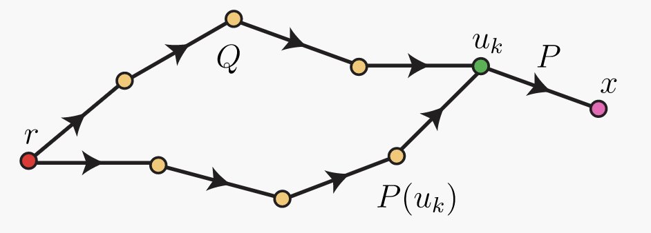
Figure 12.19. Shortest paths

By the inductive hypothesis, $δ(u_k)$ is the distance from $r$ to $u_k$, and $P(u_k)$ is a shortest path from $r$ to $u_k$. Note that $P(u_k)$ need not be the same as path $Q$, as we suggest in Figure 12.19. However, if distinct, the two paths will have the same length, namely $δ(u_k)$. Also, the distance from $r$ to $x$ is $δ(u_k)+w(u_k,x) \geq δ(u_k)$ since $P$ is a shortest path from $r$ to $x$ and $w(u_k,x)≥0$.

Let $i$ and $j$ be the unique integers for which $u_k=v_i$ and $x=v_j$. If $j<i$, then

$δ(x)=δ(v_j)≤δ(v_i)=δ(u_k)≤δ(u_k)+w(u_k)$.

Therefore the algorithm has found a path $P(x)$ from $r$ to $x$ having length $δ(x)$ which is at most the distance from $r$ to $x$. Clearly, this implies that $δ(x)$ is the distance from $r$ to $x$ and that $P(x)$ is a shortest path.

On the other hand, if $j>i$, then the inductive step at Step $i$ results in

$δ(x)≤δ(v_i)+w(v_i,y)=δ(u_k)+w(u_k,x)$.

As before, this implies that $δ(x)$ is the distance from $r$ to $x$ and that $P(x)$ is a shortest path.