15.1: Coloring the Vertices of a Square

Let's begin by coloring the vertices of a square using white and gold. If we fix the position of the square in the plane, there are \(2^4=16\) different colorings. These colorings are shown in Figure 15.1.

Figure 15.1. The 16 colorings of the vertices of a square.

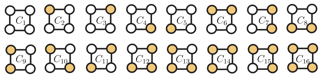
However, if we think of the square as a metal frame with a white bead or a gold bead at each corner and allow the frame to be rotated and flipped over, we realize that many of these colorings are equivalent. For instance, if we flip coloring \(C_7\) over about the vertical line dividing the square in half, we obtain coloring \(C_9\). If we rotate coloring \(C_2\) clockwise by \(90^\circ\), we obtain coloring \(C_3\). In many cases, we want to consider such equivalent colorings as a single coloring. (Recall our motivating example of necklaces made of colored beads. It makes little sense to differentiate between two necklaces if one can be rotated and flipped to become the other.)

To systematically determine how many of the colorings shown in Figure 15.1 are not equivalent, we must think about the transformations we can apply to the square and what each does to the colorings. Before examining the transformations' effects on the colorings, let's take a moment to see how they rearrange the vertices. To do this, we consider the upper-left vertex to be 1, the upper-right vertex to be 2, the lower-right vertex to be 3, and the lower-left vertex to be 4. We denote the clockwise rotation by \(90^\circ\) by \(r_1\) and see that \(r_1\) sends the vertex in position 1 to position 2, the vertex in position 2 to position 3, the vertex in position 3 to position 4, and the vertex in position 4 to position 1. For brevity, we will write \(r1(1)=2, r1(2)=3\), etc. We can also rotate the square clockwise by \(180^\circ\) and denote that rotation by \(r_2\). In this case, we find that \(r2(1)=3, r2(2)=4, r2(3)=1\), and \(r2(4)=2\). Notice that we can achieve the transformation \(r_2\) by doing \(r_1\) twice in succession. Furthermore, the clockwise rotation by \(270^\circ]), \(r_3\), can be achieved by doing \(r_1\) three times in succession. (Counterclockwise rotations can be avoided by noting that they have the same effect as a clockwise rotation, although by a different angle.)

When it comes to flipping the square, there are four axes about which we can flip it: vertical, horizontal, positive-slope diagonal, and negative-slope diagonal. We denote these flips by \(v, h, p\), and \(n\), respectively. Now notice that \(v(1)=2, v(2)=1, v(3)=4\), and \(v(4)=3\). For the flip about the horizontal axis, we have \(h(1)=4, h(2)=3, h(3)=2\), and \(h(4)=1\). For \(p\), we have \(p(1)=3, p(2)=2, p(3)=1\), and \(p(4)=4\). Finally, for \(n\) we find \(n(1)=1, n(2)=4, n(3)=3\), and \(n(4)=2\). There is one more transformation that we must mention; the transformation that does nothing to the square is called the identity transformation, denoted \(ι\). It has \(ι(1)=1, ι(2)=2, ι(3)=3\), and \(ι(4)=4\).

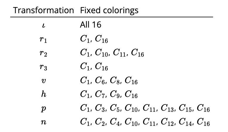
Now that we've identified the eight transformations of the square, let's make a table showing which colorings from Figure 15.1 are left unchanged by the application of each transformation. Not surprisingly, the identity transformation leaves all of the colorings unchanged. Because \(r_1\) moves the vertices cyclically, we see that only \(C_1\) and \(C_{16}\) remain unchanged when it is applied. Any coloring with more than one color would have a vertex of one color moved to one of the other color. Let's consider which colorings are fixed by \(v\), the flip about the vertical axis. For this to happen, the color at position 1 must be the same as the color at position 2, and the color at position 3 must be the same as the color at position 4. Thus, we would expect to find \(2 \cdot 2=4\) colorings unchanged by \(v\). Examining Figure 15.1, we see that these colorings are \(C_1, C_6, C_8\), and \(C_{16}\). Performing a similar analysis for the remaining five transformations leads to Figure 15.2.

Figure 15.2. Colorings fixed by transformations of the square

At this point, it's natural to ask where this is going. After all, we're trying to count the number of nonequivalent colorings, and Figure 15.2 makes no effort to group colorings based on how a transformation changes one coloring to another. It turns out that there is a useful connection between counting the nonequivalent colorings and determining the number of colorings fixed by each transformation. To develop this connection, we first need to discuss the equivalence relation created by the action of the transformations of the square on the set \(\mathcal{C}\) of all 2-colorings of the square. (Refer to Section B.13 for a refresher on the definition of equivalence relation.) To do this, notice that applying a transformation to a square with colored vertices results in another square with colored vertices. For instance, applying the transformation \(r_1\) to a square colored as in \(C_{12}\) results in a square colored as in \(C_{13}\). We say that the transformations of the square act on the set \(\mathcal{C}\) of colorings. We denote this action by adding a star to the transformation name. For instance, \(r_1^∗(C_{12})=C_{13}\) and \(v^∗(C_{10})=C_{11}\).

If \(τ\) is a transformation of the square with \(τ^∗(C_i)=C_j\), then we say colorings \(C_i\) and \(C_j\) are equivalent and write \(C_i~C_j\). Since \(ι^∗(C)=C\) for all \(C∈ \mathcal{C}\), ~ is reflexive. If \(τ_1^∗(C_i)=C_j\) and \(τ_2^∗(C_j)=C_k\), then \(τ_2^∗(τ_1^∗(C_i))=C_k\), so ~ is transitive. To complete our verification that ∼ is an equivalence relation, we must establish that it is symmetric. For this, we require the notion of the inverse of a transformation \(τ\), which is simply the transformation τ−1 that undoes whatever \(τ\) did. For instance, the inverse of \(r_1\) is the counterclockwise rotation by \(90^\circ\), which has the same effect on the location of the vertices as \(r_3\). If \(τ^∗(C_i)=C_j\), then \(τ^{−1∗}(C_j)=C_i\), so ~ is symmetric.

Before proceeding to establish the connection between the number of nonequivalent colorings (equivalence classes under ~) and the number of colorings fixed by a transformation in full generality, let's see how it looks for our example. In looking at Figure 15.1, you should notice that ~ partitions \(\mathcal{C}\) into six equivalence classes. Two contain one coloring each (the all white and all gold colorings). One contains two colorings (\(C_{10}\) and \(C_{11}\)). Finally, three contain four colorings each (one gold vertex, one white vertex, and the remaining four with two vertices of each color). Now look again at Figure 15.2 and add up the number of colorings fixed by each transformation. In doing this, we obtain 48, and when 48 is divided by the number of transformations (8), we get 6 (the number of equivalence classes)! It turns out that this is far from a fluke, as we will soon see. First, however, we introduce the concept of a permutation group to generalize our set of transformations of the square.