8.3: Properties of Green's Functions

We have noted some properties of Green’s functions in the last section. In this section we will elaborate on some of these properties as a tool for quickly constructing Green’s functions for boundary value problems. Here is a list of the properties based upon our previous solution.

Properties of the Green's Function

1. Differential Equation:

\(\dfrac{\partial}{\partial x}\left(p(x) \dfrac{\partial G(x, \xi)}{\partial x}\right)+q(x) G(x, \xi)=0, x \neq \xi\)

For \(x<\xi\) we are on the second branch and \(G(x, \xi)\) is proportional to \(y_{1}(x)\). Thus, since \(y_{1}(x)\) is a solution of the homogeneous equation, then so is \(G(x, \xi)\). For \(x>\xi\) we are on the first branch and \(G(x, \xi)\) is proportional to \(y_{2}(x)\). So, once again \(G(x, \xi)\) is a solution of the homogeneous problem.

2. Boundary Conditions:

For \(x=a\) we are on the second branch and \(G(x, \xi)\) is proportional to \(y_{1}(x)\). Thus, whatever condition \(y_{1}(x)\) satisfies, \(G(x, \xi)\) will satisfy. A similar statement can be made for \(x=b\).

3. Symmetry or Reciprocity: \(G(x, \xi)=G(\xi, x)\)

We had shown this in the last section.

4. Continuity of \(\mathbf{G}\) at \(x=\xi\): \(G\left(\xi^{+}, \xi\right)=G\left(\xi^{-}, \xi\right)\)

Here we have defined

\begin{aligned}
&G\left(\xi^{+}, x\right)=\lim _{x \downarrow \xi} G(x, \xi), \quad x>\xi \\
&G\left(\xi^{-}, x\right)=\lim _{x \uparrow \xi} G(x, \xi), \quad x<\xi
\end{aligned}

Setting \(x=\xi\) in both branches, we have

\[\dfrac{y_{1}(\xi) y_{2}(\xi)}{p W}=\dfrac{y_{1}(\xi) y_{2}(\xi)}{p W} \nonumber \]

5. Jump Discontinuity of \(\dfrac{\partial G}{\partial x}\) at \(x=\xi\):

\[\dfrac{\partial G\left(\xi^{+}, \xi\right)}{\partial x}-\dfrac{\partial G\left(\xi^{-}, \xi\right)}{\partial x}=\dfrac{1}{p(\xi)} \nonumber \]

This case is not as obvious. We first compute the derivatives by noting which branch is involved and then evaluate the derivatives and subtract them. Thus, we have

\[\begin{aligned}
\dfrac{\partial G\left(\xi^{+}, \xi\right)}{\partial x}-\dfrac{\partial G\left(\xi^{-}, \xi\right)}{\partial x} &=-\dfrac{1}{p W^{\prime}} y_{1}(\xi) y_{2}^{\prime}(\xi)+\dfrac{1}{p W} y_{1}^{\prime}(\xi) y_{2}(\xi) \\
&=-\dfrac{y_{1}^{\prime}(\xi) y_{2}(\xi)-y_{1}(\xi) y_{2}^{\prime}(\xi)}{p(\xi)\left(y_{1}(\xi) y_{2}^{\prime}(\xi)-y_{1}^{\prime}(\xi) y_{2}(\xi)\right)} \\
&=\dfrac{1}{p(\xi)}
\end{aligned} \label{8.47} \]

We now show how a knowledge of these properties allows one to quickly construct a Green’s function.

Example 8.5. Construct the Green's function for the problem

\begin{gathered}
y^{\prime \prime}+\omega^{2} y=f(x), \quad 0<x<1, \\
y(0)=0=y(1),
\end{gathered}

with \(\omega \neq 0\).

I. Find solutions to the homogeneous equation.

A general solution to the homogeneous equation is given as

\[y_{h}(x)=c_{1} \sin \omega x+c_{2} \cos \omega x . \nonumber \]

Thus, for \(x \neq \xi\),

\[G(x, \xi)=c_{1}(\xi) \sin \omega x+c_{2}(\xi) \cos \omega x \nonumber \]

II. Boundary Conditions.

First, we have \(G(0, \xi)=0\) for \(0 \leq x \leq \xi\). So,

\[G(0, \xi)=c_{2}(\xi) \cos \omega x=0 \nonumber \]

So,

\[G(x, \xi)=c_{1}(\xi) \sin \omega x, \quad 0 \leq x \leq \xi . \nonumber \]

Second, we have \(G(1, \xi)=0\) for \(\xi \leq x \leq 1\). So,

\[G(1, \xi)=c_{1}(\xi) \sin \omega+c_{2}(\xi) \cos \omega .=0 \nonumber \]

A solution can be chosen with

\[c_{2}(\xi)=-c_{1}(\xi) \tan \omega \nonumber \]

This gives

\[G(x, \xi)=c_{1}(\xi) \sin \omega x-c_{1}(\xi) \tan \omega \cos \omega x . \nonumber \]

This can be simplified by factoring out the \(c_{1}(\xi)\) and placing the remaining terms over a common denominator. The result is

\[\begin{aligned}
G(x, \xi) &=\dfrac{c_{1}(\xi)}{\cos \omega}[\sin \omega x \cos \omega-\sin \omega \cos \omega x] \\
&=-\dfrac{c_{1}(\xi)}{\cos \omega} \sin \omega(1-x)
\end{aligned} \label{8.48} \]

Since the coefficient is arbitrary at this point, as can write the result as

\[G(x, \xi)=d_{1}(\xi) \sin \omega(1-x), \quad \xi \leq x \leq 1 \nonumber \]

We note that we could have started with \(y_{2}(x)=\sin \omega(1-x)\) as one of our linearly independent solutions of the homogeneous problem in anticipation that \(y_{2}(x)\) satisfies the second boundary condition.

III. Symmetry or Reciprocity

We now impose that \(G(x, \xi)=G(\xi, x)\). To this point we have that

\(G(x, \xi)=\left\{\begin{array}{cc}
c_{1}(\xi) \sin \omega x, & 0 \leq x \leq \xi \\
d_{1}(\xi) \sin \omega(1-x), & \xi \leq x \leq 1
\end{array} .\right.\)

We can make the branches symmetric by picking the right forms for \(c_{1}(\xi)\) and \(d_{1}(\xi)\). We choose \(c_{1}(\xi)=C \sin \omega(1-\xi)\) and \(d_{1}(\xi)=C \sin \omega \xi .\) Then,

\(G(x, \xi)=\left\{\begin{array}{l}
C \sin \omega(1-\xi) \sin \omega x, 0 \leq x \leq \xi \\
C \sin \omega(1-x) \sin \omega \xi, \xi \leq x \leq 1
\end{array} .\right.\)

Now the Green's function is symmetric and we still have to determine the constant \(C\). We note that we could have gotten to this point using the Method of Variation of Parameters result where \(C=\dfrac{1}{p W}\).

IV. Continuity of \(G(x, \xi)\)

We note that we already have continuity by virtue of the symmetry imposed in the last step.

V. Jump Discontinuity in \(\dfrac{\partial}{\partial x} G(x, \xi)\).

We still need to determine \(C\). We can do this using the jump discontinuity of the derivative:

\[\dfrac{\partial G\left(\xi^{+}, \xi\right)}{\partial x}-\dfrac{\partial G\left(\xi^{-}, \xi\right)}{\partial x}=\dfrac{1}{p(\xi)} \nonumber \]

For our problem \(p(x)=1\). So, inserting our Green's function, we have

\[\begin{aligned}
1 &=\dfrac{\partial G\left(\xi^{+}, \xi\right)}{\partial x}-\dfrac{\partial G\left(\xi^{-}, \xi\right)}{\partial x} \\
&=\dfrac{\partial}{\partial x}[C \sin \omega(1-x) \sin \omega \xi]_{x=\xi}-\dfrac{\partial}{\partial x}[C \sin \omega(1-\xi) \sin \omega x]_{x=\xi} \\
&=-\omega C \cos \omega(1-\xi) \sin \omega \xi-\omega C \sin \omega(1-\xi) \cos \omega \xi \\
&=-\omega C \sin \omega(\xi+1-\xi) \\
&=-\omega C \sin \omega .
\end{aligned} \label{8.49} \]

Therefore,

\[C=-\dfrac{1}{\omega \sin \omega} . \nonumber \]

Finally, we have our Green’s function:

\[G(x, \xi)=\left\{\begin{array}{l}
-\dfrac{\sin \omega(1-\xi) \sin \omega x}{\omega \sin \omega}, 0 \leq x \leq \xi \\
-\dfrac{\sin \omega(1-x) \sin \omega \xi}{\omega \sin \omega}, \xi \leq x \leq 1
\end{array} .\right. \label{8.50} \]

It is instructive to compare this result to the Variation of Parameters result. We have the functions \(y_{1}(x)=\sin \omega x\) and \(y_{2}(x)=\sin \omega(1-x)\) as the solutions of the homogeneous equation satisfying \(y_{1}(0)=0\) and \(y_{2}(1)=0\). We need to compute \(p W\):

\[\begin{aligned}
p(x) W(x) &=y_{1}(x) y_{2}^{\prime}(x)-y_{1}^{\prime}(x) y_{2}(x) \\
&=-\omega \sin \omega x \cos \omega(1-x)-\omega \cos \omega x \sin \omega(1-x) \\
&=-\omega \sin \omega
\end{aligned} \label{8.51} \]

Inserting this result into the Variation of Parameters result for the Green’s function leads to the same Green’s function as above.

8.3.1 The Dirac Delta Function

We will develop a more general theory of Green's functions for ordinary differential equations which encompasses some of the listed properties. The Green's function satisfies a homogeneous differential equation for \(x \neq \xi\),

\[\dfrac{\partial}{\partial x}\left(p(x) \dfrac{\partial G(x, \xi)}{\partial x}\right)+q(x) G(x, \xi)=0, \quad x \neq \xi . \label{8.52} \]

When \(x=\xi\), we saw that the derivative has a jump in its value. This is similar to the step, or Heaviside, function,

\(H(x)=\left\{\begin{array}{l}
1, x>0 \\
0, x<0
\end{array}\right.\)

In the case of the step function, the derivative is zero everywhere except at the jump. At the jump, there is an infinite slope, though technically, we have learned that there is no derivative at this point. We will try to remedy this by introducing the Dirac delta function,

\[\delta(x)=\dfrac{d}{d x} H(x) . \nonumber \]

We will then show that the Green’s function satisfies the differential equation

\[\dfrac{\partial}{\partial x}\left(p(x) \dfrac{\partial G(x, \xi)}{\partial x}\right)+q(x) G(x, \xi)=\delta(x-\xi) . \label{8.53} \]

The Dirac delta function, \(\delta(x)\), is one example of what is known as a generalized function, or a distribution. Dirac had introduced this function in the 1930's in his study of quantum mechanics as a useful tool. It was later studied in a general theory of distributions and found to be more than a simple tool used by physicists. The Dirac delta function, as any distribution, only makes sense under an integral.

Before defining the Dirac delta function and introducing some of its properties, we will look at some representations that lead to the definition. We will consider the limits of two sequences of functions.

First we define the sequence of functions

\(f_{n}(x)=\left\{\begin{array}{l}
0,|x|>\dfrac{1}{n} \\
\dfrac{n}{2},|x|<\dfrac{1}{n}
\end{array}\right.\)

This is a sequence of functions as shown in Figure 8.1. As \(n \rightarrow \infty\), we find the limit is zero for \(x \neq 0\) and is infinite for \(x=0\). However, the area under each member of the sequences is one since each box has height \(\dfrac{n}{2}\) and width \(\dfrac{2}{n}\). Thus, the limiting function is zero at most points but has area one. (At this point the reader who is new to this should be doing some head scratching!)

Figure 8.1. A plot of the functions \(f_{n}(x)\) for \(n=2,4,8\).

The limit is not really a function. It is a generalized function. It is called the Dirac delta function, which is defined by

1. \(\delta(x)=0\) for \(x \neq 0\).
2. \(\int_{-\infty}^{\infty} \delta(x) d x=1\).

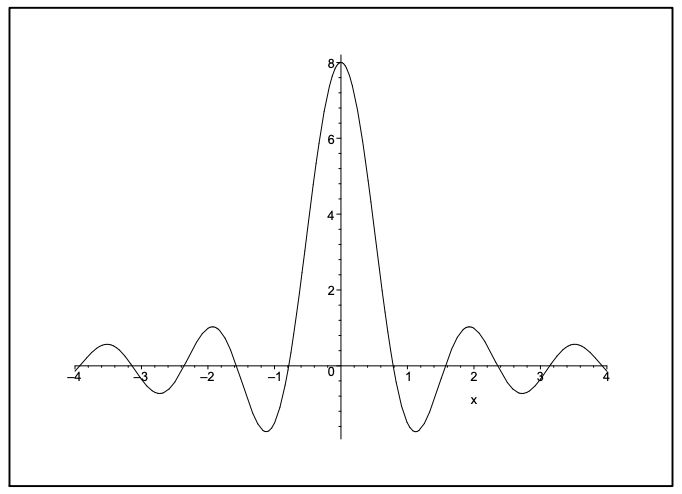
Another example is the sequence defined by

\[D_{n}(x)=\dfrac{2 \sin n x}{x} . \label{8.54} \]

We can graph this function. We first rewrite this function as

\[D_{n}(x)=2 n \dfrac{\sin n x}{n x} . \nonumber \]

Now it is easy to see that as \(x \rightarrow 0, D_{n}(x) \rightarrow 2 n\). For large \(x\), The function tends to zero. A plot of this function is in Figure 8.2. For large \(n\) the peak grows and the values of \(D_{n}(x)\) for \(x \neq 0\) tend to zero as show in Figure 8.3.
We note that in the limit \(n \rightarrow \infty, D_{n}(x)=0\) for \(x \neq 0\) and it is infinite at \(x=0\). However, using complex analysis one can show that the area is

\[\int_{-\infty}^{\infty} D_{n}(x) d x=2 \pi \nonumber \]

Thus, the area is constant for each \(n\).

Figure 8.2. A plot of the function \(D_n(x)\) for \(n = 4\).

Figure 8.3. A plot of the function \(D_n(x)\) for \(n = 40\).

There are two main properties that define a Dirac delta function. First one has that the area under the delta function is one,

\[\int_{-\infty}^{\infty} \delta(x) d x=1 \nonumber \]

Integration over more general intervals gives

\[\int_{a}^{b} \delta(x) d x=1, \quad 0 \in[a, b] \nonumber \]

and

\[\int_{a}^{b} \delta(x) d x=0, \quad 0 \notin[a, b] . \nonumber \]

Another common property is what is sometimes called the sifting property. Namely, integrating the product of a function and the delta function “sifts” out a specific value of the function. It is given by

\[\int_{-\infty}^{\infty} \delta(x-a) f(x) d x=f(a) \nonumber \]

This can be seen by noting that the delta function is zero everywhere except at \(x=a\). Therefore, the integrand is zero everywhere and the only contribution from \(f(x)\) will be from \(x=a\). So, we can replace \(f(x)\) with \(f(a)\) under the integral. Since \(f(a)\) is a constant, we have that

\[\int_{-\infty}^{\infty} \delta(x-a) f(x) d x=\int_{-\infty}^{\infty} \delta(x-a) f(a) d x=f(a) \int_{-\infty}^{\infty} \delta(x-a) d x=f(a) . \nonumber \]

Another property results from using a scaled argument, \(a x\). In this case we show that

\[\delta(a x)=|a|^{-1} \delta(x) . \label{8.55} \]

As usual, this only has meaning under an integral sign. So, we place \(\delta(a x)\) inside an integral and make a substitution \(y=a x\):

\[\begin{aligned}
\int_{-\infty}^{\infty} \delta(a x) d x &=\lim _{L \rightarrow \infty} \int_{-L}^{L} \delta(a x) d x \\
&=\lim _{L \rightarrow \infty} \dfrac{1}{a} \int_{-a L}^{a L} \delta(y) d y
\end{aligned} \label{8.56} \]

If \(a>0\) then

\[\int_{-\infty}^{\infty} \delta(a x) d x=\dfrac{1}{a} \int_{-\infty}^{\infty} \delta(y) d y . \nonumber \]

However, if \(a<0\) then

\[\int_{-\infty}^{\infty} \delta(a x) d x=\dfrac{1}{a} \int_{\infty}^{-\infty} \delta(y) d y=-\dfrac{1}{a} \int_{-\infty}^{\infty} \delta(y) d y . \nonumber \]

The overall difference in a multiplicative minus sign can be absorbed into one expression by changing the factor \(1 / a\) to \(1 /|a|\). Thus,

\[\int_{-\infty}^{\infty} \delta(a x) d x=\dfrac{1}{|a|} \int_{-\infty}^{\infty} \delta(y) d y . \label{8.57} \]

Example 8.6. Evaluate \(\in_{-\infty}^{\infty}(5x+1) \delta(4(x-2))dx\). This is a straight forward integration:

\[\int_{-\infty}^{\infty}(5 x+1) \delta(4(x-2)) d x=\dfrac{1}{4} \int_{-\infty}^{\infty}(5 x+1) \delta(x-2) d x=\dfrac{11}{4} \nonumber \]

A more general scaling of the argument takes the form \(\delta(f(x))\). The integral of \(\delta(f(x))\) can be evaluated depending upon the number of zeros of \(f(x)\). If there is only one zero, \(f\left(x_{1}\right)=0\), then one has that

\[\int_{-\infty}^{\infty} \delta(f(x)) d x=\int_{-\infty}^{\infty} \dfrac{1}{\left|f^{\prime}\left(x_{1}\right)\right|} \delta\left(x-x_{1}\right) d x \nonumber \]

This can be proven using the substitution \(y=f(x)\) and is left as an exercise for the reader. This result is often written as

\[\delta(f(x))=\dfrac{1}{\left|f^{\prime}\left(x_{1}\right)\right|} \delta\left(x-x_{1}\right) . \nonumber \]

Example 8.7. Evaluate \(\int_{-\infty}^{\infty} \delta(3x-2)x^2dx\).

This is not a simple \(\delta(x-a)\). So, we need to find the zeros of \(f(x)=3 x-2\). There is only one, \(x=\dfrac{2}{3}\). Also, \(\left|f^{\prime}(x)\right|=3\). Therefore, we have

\[\int_{-\infty}^{\infty} \delta(3 x-2) x^{2} d x=\int_{-\infty}^{\infty} \dfrac{1}{3} \delta\left(x-\dfrac{2}{3}\right) x^{2} d x=\dfrac{1}{3}\left(\dfrac{2}{3}\right)^{2}=\dfrac{4}{27} \nonumber \]

Note that this integral can be evaluated the long way by using the substitution \(y=3 x-2\). Then, \(d y=3 d x\) and \(x=(y+2) / 3\). This gives

\[\int_{-\infty}^{\infty} \delta(3 x-2) x^{2} d x=\dfrac{1}{3} \int_{-\infty}^{\infty} \delta(y)\left(\dfrac{y+2}{3}\right)^{2} d y=\dfrac{1}{3}\left(\dfrac{4}{9}\right)=\dfrac{4}{27} . \nonumber \]

More generally, one can show that when \(f\left(x_{j}\right)=0\) and \(f^{\prime}\left(x_{j}\right) \neq 0\) for \(x_{j}\), \(j=1,2, \ldots, n\), (i.e.; when one has $n$ simple zeros), then

\[\delta(f(x))=\sum_{j=1}^{n} \dfrac{1}{\left|f^{\prime}\left(x_{j}\right)\right|} \delta\left(x-x_{j}\right) . \nonumber \]

Example 8.8. Evaluate \(\int_0^{2 \pi} \cos x \delta \left( x^2 - \pi^2 \right)dx\).

In this case the argument of the delta function has two simple roots. Namely, \(f(x)=x^{2}-\pi^{2}=0\) when \(x=\pm \pi\). Furthermore, \(f^{\prime}(x)=2 x\). Therefore, \(\left|f^{\prime}(\pm \pi)\right|=2 \pi\). This gives

\[\delta\left(x^{2}-\pi^{2}\right)=\dfrac{1}{2 \pi}[\delta(x-\pi)+\delta(x+\pi)] . \nonumber \]

Inserting this expression into the integral and noting that \(x=-\pi\) is not in the integration interval, we have

\[\begin{aligned}
\int_{0}^{2 \pi} \cos x \delta\left(x^{2}-\pi^{2}\right) d x &=\dfrac{1}{2 \pi} \int_{0}^{2 \pi} \cos x[\delta(x-\pi)+\delta(x+\pi)] d x \\
&=\dfrac{1}{2 \pi} \cos \pi=-\dfrac{1}{2 \pi}
\end{aligned} \label{8.58} \]

Finally, we previously noted there is a relationship between the Heaviside, or step, function and the Dirac delta function. We defined the Heaviside function as

\(H(x)=\left\{\begin{array}{l}
0, x<0 \\
1, x>0
\end{array}\right.\)

Then, it is easy to see that \(H^{\prime}(x)=\delta(x)\).

8.3.2 Green’s Function Differential Equation

As noted, the Green’s function satisfies the differential equation

\[\dfrac{\partial}{\partial x}\left(p(x) \dfrac{\partial G(x, \xi)}{\partial x}\right)+q(x) G(x, \xi)=\delta(x-\xi) \label{8.59} \]

and satisfies homogeneous conditions. We have used the Green’s function to solve the nonhomogeneous equation

\[\dfrac{d}{d x}\left(p(x) \dfrac{d y(x)}{d x}\right)+q(x) y(x)=f(x) . \label{8.60} \]

These equations can be written in the more compact forms

\[\begin{gathered}
\mathcal{L}[y]=f(x) \\
\mathcal{L}[G]=\delta(x-\xi) .
\end{gathered} \label{8.61} \]

Multiplying the first equation by \(G(x, \xi)\), the second equation by \(y(x)\), and then subtracting, we have

\[G \mathcal{L}[y]-y \mathcal{L}[G]=f(x) G(x, \xi)-\delta(x-\xi) y(x) . \nonumber \]

Now, integrate both sides from \(x=a\) to \(x=b\). The left side becomes

\[\int_{a}^{b}[f(x) G(x, \xi)-\delta(x-\xi) y(x)] d x=\int_{a}^{b} f(x) G(x, \xi) d x-y(\xi) \nonumber \]

and, using Green's Identity, the right side is

\[\int_{a}^{b}(G \mathcal{L}[y]-y \mathcal{L}[G]) d x=\left[p(x)\left(G(x, \xi) y^{\prime}(x)-y(x) \dfrac{\partial G}{\partial x}(x, \xi)\right)\right]_{x=a}^{x=b} \nonumber \]

Combining these results and rearranging, we obtain

\[y(\xi)=\int_{a}^{b} f(x) G(x, \xi) d x-\left[p(x)\left(y(x) \dfrac{\partial G}{\partial x}(x, \xi)-G(x, \xi) y^{\prime}(x)\right)\right]_{x=a}^{x=b} \label{8.62} \]

Next, one uses the boundary conditions in the problem in order to determine which conditions the Green's function needs to satisfy. For example, if we have the boundary condition \(y(a)=0\) and \(y(b)=0\), then the boundary terms yield

\[\begin{aligned}
y(\xi)=& \int_{a}^{b} f(x) G(x, \xi) d x-\left[p(b)\left(y(b) \dfrac{\partial G}{\partial x}(b, \xi)-G(b, \xi) y^{\prime}(b)\right)\right] \\
&+\left[p(a)\left(y(a) \dfrac{\partial G}{\partial x}(a, \xi)-G(a, \xi) y^{\prime}(a)\right)\right] \\
=& \int_{a}^{b} f(x) G(x, \xi) d x+p(b) G(b, \xi) y^{\prime}(b)-p(a) G(a, \xi) y^{\prime}(a) .
\end{aligned} \label{8.63} \]

The right hand side will only vanish if \(G(x, \xi)\) also satisfies these homogeneous boundary conditions. This then leaves us with the solution

\[y(\xi)=\int_{a}^{b} f(x) G(x, \xi) d x . \nonumber \]

We should rewrite this as a function of \(x\). So, we replace \(\xi\) with \(x\) and \(x\) with \(\xi\). This gives

\[y(x)=\int_{a}^{b} f(\xi) G(\xi, x) d \xi . \nonumber \]

However, this is not yet in the desirable form. The arguments of the Green's function are reversed. But, \(G(x, \xi)\) is symmetric in its arguments. So, we can simply switch the arguments getting the desired result.

We can now see that the theory works for other boundary conditions. If we had \(y^{\prime}(a)=0\), then the \(y(a) \dfrac{\partial G}{\partial x}(a, \xi)\) term in the boundary terms could be made to vanish if we set \(\dfrac{\partial G}{\partial x}(a, \xi)=0\). So, this confirms that other boundary value problems can be posed besides the one elaborated upon in the chapter so far.

We can even adapt this theory to nonhomogeneous boundary conditions. We first rewrite Equation (8.62) as

\[y(x)=\int_{a}^{b} G(x, \xi) f(\xi) d \xi-\left[p(\xi)\left(y(\xi) \dfrac{\partial G}{\partial \xi}(x, \xi)-G(x, \xi) y^{\prime}(\xi)\right)\right]_{\xi=a}^{\xi=b} . \label{8.64} \]

Let's consider the boundary conditions \(y(a)=\alpha\) and \(y^{\prime}(b)= beta\). We also assume that \(G(x, \xi)\) satisfies homogeneous boundary conditions,

\[G(a, \xi)=0, \quad \dfrac{\partial G}{\partial \xi}(b, \xi)=0 . \nonumber \]

in both \(x\) and \(\xi\) since the Green's function is symmetric in its variables. Then, we need only focus on the boundary terms to examine the effect on the solution. We have

\[\begin{aligned}
{\left[p(\xi)\left(y(\xi) \dfrac{\partial G}{\partial \xi}(x, \xi)-G(x, \xi) y^{\prime}(\xi)\right)\right]_{\xi=a}^{\xi=b} } &=\left[p(b)\left(y(b) \dfrac{\partial G}{\partial \xi}(x, b)-G(x, b) y^{\prime}(b)\right)\right] \\
&-\left[p(a)\left(y(a) \dfrac{\partial G}{\partial \xi}(x, a)-G(x, a) y^{\prime}(a)\right)\right.\\
&=-\beta p(b) G(x, b)-\alpha p(a) \dfrac{\partial G}{\partial \xi}(x, a)
\end{aligned} \label{8.65} \]

Therefore, we have the solution

\[y(x)=\int_{a}^{b} G(x, \xi) f(\xi) d \xi+\beta p(b) G(x, b)+\alpha p(a) \dfrac{\partial G}{\partial \xi}(x, a) . \label{8.66} \]

This solution satisfies the nonhomogeneous boundary conditions. Let’s see how it works.

Example  8.9. Modify Example 8.4. to solve the boundary value problem \(y'' = x^2, \quad y(0)=1, y(1)=2\) using the boundary value Green's function that we found:

\[G(x, \xi)=\left\{\begin{array}{l}
-\xi(1-x), 0 \leq \xi \leq x \\
-x(1-\xi), x \leq \xi \leq 1
\end{array} .\right. \label{8.67} \]

We insert the Green’s function into the solution and use the given conditions to obtain

\[\begin{aligned}
y(x) &=\int_{0}^{1} G(x, \xi) \xi^{2} d \xi-\left[y(\xi) \dfrac{\partial G}{\partial \xi}(x, \xi)-G(x, \xi) y^{\prime}(\xi)\right]_{\xi=0}^{\xi=1} \\
&=\int_{0}^{x}(x-1) \xi^{3} d \xi+\int_{x}^{1} x(\xi-1) \xi^{2} d \xi+y(0) \dfrac{\partial G}{\partial \xi}(x, 0)-y(1) \dfrac{\partial G}{\partial \xi}(x, 1) \\
&=\dfrac{(x-1) x^{4}}{4}+\dfrac{x\left(1-x^{4}\right)}{4}-\dfrac{x\left(1-x^{3}\right)}{3}+(x-1)-2 x \\
&=\dfrac{x^{4}}{12}+\dfrac{35}{12} x-1
\end{aligned} \label{8.68} \]

Of course, this problem can be solved more directly by direct integration. The general solution is

\[y(x)=\dfrac{x^{4}}{12}+c_{1} x+c_{2} . \nonumber \]

Inserting this solution into each boundary condition yields the same result.

We have seen how the introduction of the Dirac delta function in the differential equation satisfied by the Green's function, Equation (8.59), can lead to the solution of boundary value problems. The Dirac delta function also aids in our interpretation of the Green's function. We note that the Green's function is a solution of an equation in which the nonhomogeneous function is \(\delta(x-\xi)\). Note that if we multiply the delta function by \(f(\xi)\) and integrate we obtain

\[\int_{-\infty}^{\infty} \delta(x-\xi) f(\xi) d \xi=f(x) \nonumber \]

We can view the delta function as a unit impulse at \(x=\xi\) which can be used to build \(f(x)\) as a sum of impulses of different strengths, \(f(\xi)\). Thus, the Green's function is the response to the impulse as governed by the differential equation and given boundary conditions.

In particular, the delta function forced equation can be used to derive the jump condition. We begin with the equation in the form

\[\dfrac{\partial}{\partial x}\left(p(x) \dfrac{\partial G(x, \xi)}{\partial x}\right)+q(x) G(x, \xi)=\delta(x-\xi) . \label{8.69} \]

Now, integrate both sides from \(\xi-\epsilon\) to \(\xi+\epsilon\) and take the limit as \(\epsilon \rightarrow 0\). Then,

\[\begin{aligned}
\lim _{\epsilon \rightarrow 0} \int_{\xi-\epsilon}^{\xi+\epsilon}\left[\dfrac{\partial}{\partial x}\left(p(x) \dfrac{\partial G(x, \xi)}{\partial x}\right)+q(x) G(x, \xi)\right] d x &=\lim _{\epsilon \rightarrow 0} \int_{\xi-\epsilon}^{\xi+\epsilon} \delta(x-\xi) d x \\
&=1 .
\end{aligned} \label{8.70} \]

Since the \(q(x)\) term is continuous, the limit of that term vanishes. Using the Fundamental Theorem of Calculus, we then have

\[\lim _{\epsilon \rightarrow 0}\left[p(x) \dfrac{\partial G(x, \xi)}{\partial x}\right]_{\xi-\epsilon}^{\xi+\epsilon}=1 . \label{8.71} \]

This is the jump condition that we have been using!