11.4: Modelling the eye–revisited

Let me return to my model of the eye. With the function \(P_n(\cos\theta)\) as the solution to the angular equation, we find that the solutions to the radial equation are

\[R=Ar^n + Br^{-n-1}.\]

The singular part is not acceptable, so once again we find that the solution takes the form

\[u(r,\theta) = \sum_{n=0}^\infty A_n r^n P_n(\cos\theta)\]

We now need to impose the boundary condition that the temperature is \(20^\circ\) C in an opening angle of \(45^\circ\), and \(36^\circ\) elsewhere. This leads to the equation

\[\begin{aligned} \sum_{n=0}^\infty A_n c^n P_n(\cos\theta) = \left\{ \begin{array}{ll} 20 & 0<\theta<\pi/4\\ 36 & \pi/4 < \theta < \pi \end{array}\right.\end{aligned}\]

This leads to the integral, after once again changing to \(x=\cos\theta\),

\[A_n = \frac{2n+1}{2} \left[\int_{-1}^1 36 P_n(x) dx -\int_{\frac{1}{2}\sqrt{2}}^1 16 P_n(x) dx\right].\]

These integrals can easily be evaluated, and a sketch for the temperature can be found in figure \(\PageIndex{1}\).

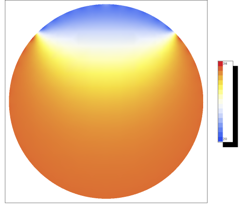
Figure \(\PageIndex{1}\): A cross-section of the temperature in the eye. We have summed over the first 40 Legendre polynomials.

Notice that we need to integrate over \(x=\cos\theta\) to obtain the coefficients \(A_n\). The integration over \(\theta\) in spherical coordinates is \(\int_0^\pi \sin \theta d\theta = \int_{-1}^1 1 dx\), and so automatically implies that \(\cos\theta\) is the right variable to use, as also follows from the orthogonality of \(P_n(x)\).