7.2: Coupled First-Order Equations

We now consider the general system of differential equations given by $$\label{eq:1}\overset{.}{x}_1=ax_1+bx_2,\quad\overset{.}{x}_2=cx_1+dx_2,$$ which can be written using vector notation as $$\label{eq:2}\overset{.}{\mathbf{x}}=\mathbf{Ax}.$$

Before solving this system of odes using matrix techniques, I first want to show that we could actually solve these equations by converting the system into a single second-order equation. We take the derivative of the first equation and use both equations to write $$\begin{aligned}\overset{..}{x}_1&=a\overset{.}{x}_1+b\overset{.}{x}_2 \\ &=a\overset{.}{x}_1+b(cx_1+dx_2) \\ &=a\overset{.}{x}_1+bcx_1+d(\overset{.}{x}_1-ax_1) \\ &=(a+d)\overset{.}{x}_1-(ad-bc)x_1.\end{aligned}$$

The system of two first-order equations therefore becomes the following second-order equation:

$$\overset{..}{x}_1-(a+d)\overset{.}{x}_1+(ad-bc)x_1=0.\nonumber$$

If we had taken the derivative of the second equation instead, we would have obtained the identical equation for $x_2$:

$$\overset{..}{x}_2-(a+d)\overset{.}{x}_2+(ad-bc)x_2=0.\nonumber$$

In general, a system of $n$ first-order linear homogeneous equations can be converted into an equivalent $n$-th order linear homogeneous equation. Numerical methods usually require the conversion in reverse; that is, a conversion of an $n$-th order equation into a system of $n$ first-order equations.

With the ansatz $x_1 = e^{\lambda t}$ or $x_2 = e^{\lambda t}$, the second-order odes have the characteristic equation $$\lambda^2-(a+d)\lambda +(ad-bc)=0.\nonumber$$

This is identical to the characteristic equation obtained for the matrix $\mathbf{A}$ from an eigenvalue analysis.

We will see that $\eqref{eq:1}$ can in fact be solved by considering the eigenvalues and eigenvectors of the matrix $\mathbf{A}$. We will demonstrate the solution for three separate cases: (i) eigenvalues of $\mathbf{A}$ are real and there are two linearly independent eigenvectors; (ii) eigenvalues of $\mathbf{A}$ are complex conjugates, and; (iii) $\mathbf{A}$ has only one linearly independent eigenvector. These three cases are analogous to the cases considered previously when solving the homogeneous linear constant-coefficient second-order equation.

Distinct Real Eigenvalues

We illustrate the solution method by example.

Example $\PageIndex{1}$

Find the general solution of $\overset{.}{x}_1=x_2+x_2,\:\overset{.}{x}_2=4x_1+x_2$.

Solution

View tutorial on YouTube

The equation to be solved may be rewritten in matrix form as $$\frac{d}{dt}\left(\begin{array}{c}x_1\\x_2\end{array}\right)=\left(\begin{array}{cc}1&1\\4&1\end{array}\right)\left(\begin{array}{c}x_1\\x_2\end{array}\right),\nonumber$$ or using vector notation, written as $\eqref{eq:2}$. We take as our ansatz $\mathbf{x}(t) = \mathbf{v}e^{\lambda t}$, where $\mathbf{v}$ and $\lambda$ are independent of $t$. Upon substitution into $\eqref{eq:2}$, we obtain $$\lambda\mathbf{v}e^{\lambda t}=\mathbf{Av}e^{\lambda t};\nonumber$$ and upon cancellation of the exponential, we obtain the eigenvalue problem $$\label{eq:3}\mathbf{Av}=\lambda\mathbf{v}.$$

Finding the characteristic equation using (7.1.8), we have $$\begin{aligned}0&=\det (\mathbf{A}-\lambda\mathbf{I}) \\ &=\lambda^2-2\lambda -3 \\ &=(\lambda -3)(\lambda +1).\end{aligned}$$

Therefore, the two eigenvalues are $\lambda_1=3$ and $\lambda_2=-1$.

To determine the corresponding eigenvectors, we substitute the eigenvalues successively into $$\label{eq:4}(\mathbf{A}-\lambda\mathbf{I})\mathbf{v}=0.$$

We will write the corresponding eigenvectors $\mathbf{v_1}$ and $\mathbf{v_2}$ using the matrix notation $$\left(\begin{array}{cc}\mathbf{v_1}&\mathbf{v_2}\end{array}\right)=\left(\begin{array}{cc}v_{11}&v_{12} \\ v_{21}&v_{22}\end{array}\right),\nonumber$$ where the components of $\mathbf{v_1}$ and $\mathbf{v_2}$ are written with subscripts corresponding to the first and second columns of a $2\times 2$ matrix.

For $\lambda_1 = 3$, and unknown eigenvector $\mathbf{v_1}$, we have from $\eqref{eq:4}$ $$\begin{aligned}-2v_{11}+v_{21}&=0, \\ 4v_{11}-2v_{21}&=0.\end{aligned}$$

Clearly, the second equation is just the first equation multiplied by $−2$, so only one equation is linearly independent. This will always be true, so for the $2\times 2$ case we need only consider the first row of the matrix. The first eigenvector therefore satisfies $v_{21} = 2v_{11}$. Recall that an eigenvector is only unique up to multiplication by a constant: we may therefore take $v_{11} = 1$ for convenience.

For $\lambda_2 = −1$, and eigenvector $\mathbf{v_2} = (v_{12}, v_{22})^T$, we have from $\eqref{eq:4}$ $$2v_{12}+v_{22}=0,\nonumber$$ so that $v_{22}=-2v_{12}$. Here, we take $v_{12}=1$.

Therefore, our eigenvalues and eigenvectors are given by $$\lambda_1=3,\:\mathbf{v_1}=\left(\begin{array}{c}1\\2\end{array}\right);\quad\lambda_2=-1,\:\mathbf{v_2}=\left(\begin{array}{c}1\\-2\end{array}\right).\nonumber$$

A node may be attracting or repelling depending on whether the eigenvalues are both negative (as is the case here) or positive. Observe that the trajectories collapse onto the $\mathbf{v_2}$ eigenvector since $\lambda_1 < \lambda_2 < 0$ and decay is more rapid along the $\mathbf{v_1}$ direction.

Distinct Complex-Conjugate Eigenvalues

Example $\PageIndex{2}$

Find the general solution of $\overset{.}{x}_1=-\frac{1}{2}x_1+x_2 ,\:\overset{.}{x}_2=-x_1-\frac{1}{2}x_2$.

Solution

View tutorial on YouTube

The equations in matrix form are $$\frac{d}{dt}\left(\begin{array}{c}x_1 \\ x_2\end{array}\right)=\left(\begin{array}{cc}-\frac{1}{2}&1 \\ -1&-\frac{1}{2}\end{array}\right)\left(\begin{array}{c}x_1 \\ x_2\end{array}\right).\nonumber$$

The ansatz $\mathbf{x} = \mathbf{v}e^{\lambda t}$ leads to the equation $$\begin{aligned}0&=\det (\mathbf{A}-\lambda\mathbf{I}) \\ &=\lambda^2+\lambda +\frac{5}{4}.\end{aligned}$$

Therefore, $\lambda = −1/2 ± i$; and we observe that the eigenvalues occur as a complex conjugate pair. We will denote the two eigenvalues as $$\lambda =-\frac{1}{2}+i\quad\text{and}\quad\overline{\lambda}=-\frac{1}{2}-i.\nonumber$$

Now, for $\mathbf{A}$ a real matrix, if $\mathbf{Av} = \lambda\mathbf{v}$, then $\mathbf{A}\mathbf{\overline{v}}=\overline{\lambda}\mathbf{\overline{v}}$. Therefore, the eigenvectors also occur as a complex conjugate pair. The eigenvector $\mathbf{v}$ associated with eigenvalue $\lambda$ satisfies $−iv_1 + v_2 = 0$, and normalizing with $v_1 = 1$, we have $$\mathbf{v}=\left(\begin{array}{c}1 \\ i\end{array}\right).\nonumber$$

We have therefore determined two independent complex solutions to the ode, that is, $$\mathbf{v}e^{\lambda t}\quad\text{and}\quad\mathbf{\overline{v}}e^{\overline{\lambda}t},\nonumber$$ and we can form a linear combination of these two complex solutions to construct two independent real solutions. Namely, if the complex functions $z(t)$ and $\overline{z}(t)$ are written as $$z(t)=\text{Re }\{z(t)\}+i\text{ Im }\{z(t)\},\quad\overline{z}(t)=\text{Re }\{z(t)\}-i\text{ Im }\{z(t)\},\nonumber$$ then two real functions can be constructed from the following linear combinations of $z$ and $\overline{z}$:

$$\frac{z+\overline{z}}{2}=\text{Re }\{z(t)\}\quad\text{and}\quad\frac{z-\overline{z}}{2i}=\text{Im }\{z(t)\}.\nonumber$$

Thus the two real vector functions that can be constructed from our two complex vector functions are $$\begin{aligned}\text{Re }\{\mathbf{v}e^{\lambda t}\}&=\text{Re }\left\{\left(\begin{array}{c}1 \\ i\end{array}\right)e^{(-\frac{1}{2}+i)t}\right\} \\ &=e^{-\frac{1}{2}t}\text{Re }\left\{\left(\begin{array}{c}1\\i\end{array}\right)(\cos t+i\sin t)\right\} \\ &=e^{-\frac{1}{2}t}\left(\begin{array}{c}\cos t \\ -\sin t\end{array}\right);\end{aligned}$$

Figure $\PageIndex{1}$: Phase portrait with complex conjugate eigenvalues.

and $$\begin{aligned}\text{Im }\{\mathbf{v}e^{\lambda t}\}&=e^{-\frac{1}{2}t}\text{Im }\left\{\left(\begin{array}{c}1\\i\end{array}\right)(\cos t+i\sin t)\right\} \\ &=e^{-\frac{1}{2}t}\left(\begin{array}{c}\sin t\\ \cos t\end{array}\right).\end{aligned}$$

Taking a linear superposition of these two real solutions yields the general solution to the ode, given by $$\mathbf{x}=e^{-\frac{1}{2}t}\left(A\left(\begin{array}{c}\cos t \\-\sin t\end{array}\right)+B\left(\begin{array}{c}\sin t\\ \cos t\end{array}\right)\right).\nonumber$$

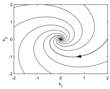
The corresponding phase portrait is shown in Fig. $\PageIndex{1}$. We say the origin is a spiral point. If the real part of the complex eigenvalue is negative, as is the case here, then solutions spiral into the origin. If the real part of the eigenvalue is positive, then solutions spiral out of the origin.

The direction of the spiral—here, it is clockwise—can be determined easily. If we examine the ode with $x_1 = 0$ and $x_2 = 1$, we see that $\overset{.}{x}_1 = 1$ and $\overset{.}{x}_2 = −1/2$. The trajectory at the point $(0, 1)$ is moving to the right and downward, and this is possible only if the spiral is clockwise. A counterclockwise trajectory would be moving to the left and downward.

Repeated Eigenvalues with One Eigenvector

Example $\PageIndex{3}$

Find the general solution of $\overset{.}{x}_1=x_1-x_2,\:\overset{.}{x}_2=x_1+3x_2$.

Solution

View tutorial on YouTube

The equations in matrix form are $$\label{eq:5}\frac{d}{dt}\left(\begin{array}{c}x_1 \\ x_2\end{array}\right)=\left(\begin{array}{cc}1&-1 \\ 1&3\end{array}\right)\left(\begin{array}{c}x_1 \\ x_2\end{array}\right).$$

The ansatz $\mathbf{x} = \mathbf{v}e^{\lambda t}$ leads to the characteristic equation $$\begin{aligned}0&=\det (\mathbf{A}-\lambda\mathbf{I}) \\ &=\lambda^2-4\lambda +4 \\ &=(\lambda -2)^2.\end{aligned}$$

Therefore, $\lambda = 2$ is a repeated eigenvalue. The associated eigenvector is found from $−v_1 − v_2 = 0$, or $v_2 = −v_1$; and normalizing with $v_1 = 1$, we have $$\lambda =2,\quad\mathbf{v}=\left(\begin{array}{c}1\\-1\end{array}\right).\nonumber$$

We have thus found a single solution to the ode, given by $$\mathbf{x_1}(t)=c_1\left(\begin{array}{c}1\\-1\end{array}\right)e^{2t},\nonumber$$ and we need to find the missing second solution to be able to satisfy the initial conditions. An ansatz of $t$ times the first solution is tempting, but will fail. Here, we will cheat and find the missing second solution by solving the equivalent secondorder, homogeneous, constant-coefficient differential equation.

We already know that this second-order differential equation for $x_1(t)$ has a characteristic equation with a degenerate eigenvalue given by $\lambda = 2$. Therefore, the general solution for $x_1$ is given by $$x_1(t)=(c_1+tc_2)e^{2t}.\nonumber$$

Since from the first differential equation, $x_2 = x_1 − \overset{.}{x}_1$, we compute $$\overset{.}{x}_1=(2c_1+(1+2t)c_2)e^{2t},\nonumber$$ so that $$\begin{aligned}x_2&=x_1-\overset{.}{x}_1 \\ &=(c_1+tc_2)e^{2t}-(2c_1+(1+2t)c_2)e^{2t} \\ &=-c_1e^{2t}+c_2(-1-t)e^{2t}.\end{aligned}$$

Combining our results for $x_1$ and $x_2$, we have therefore found $$\left(\begin{array}{c}x_1 \\ x_2\end{array}\right)=c_1\left(\begin{array}{c}1\\-1\end{array}\right)e^{2t}+c_2\left[\left(\begin{array}{c}0\\-1\end{array}\right)+\left(\begin{array}{c}1\\-1\end{array}\right)t\right]e^{2t}.\nonumber$$

Our missing linearly independent solution is thus determined to $$\label{eq:6}\mathbf{x}(t)=c_2\left[\left(\begin{array}{c}0\\-1\end{array}\right)+\left(\begin{array}{c}1\\-1\end{array}\right)t\right]e^{2t}.$$

The second term of $\eqref{eq:6}$ is just $t$ times the first solution; however, this is not sufficient. Indeed, the correct ansatz to find the second solution directly is given by $$\label{eq:7}\mathbf{x}=(\mathbf{w}+t\mathbf{v})e^{\lambda t},$$

Figure $\PageIndex{2}$: Phase portrait with only one eigenvector.

where $\lambda$ and $\mathbf{v}$ is the eigenvalue and eigenvector of the first solution, and $\mathbf{w}$ is an unknown vector to be determined. To illustrate this direct method, we substitute $\eqref{eq:7}$ into $\mathbf{\overset{.}{x}} = \mathbf{Ax}$, assuming $\mathbf{Av} = \lambda\mathbf{v}$. Canceling the exponential, we obtain $$\mathbf{v}+\lambda (\mathbf{w}+t\mathbf{v})=\mathbf{Aw}+\lambda t\mathbf{v}.\nonumber$$

Further canceling the common term $\lambda t\mathbf{v}$ and rewriting yields $$\label{eq:8}(\mathbf{A}-\lambda\mathbf{I})\mathbf{w}=\mathbf{v}.$$

If $\mathbf{A}$ has only a single linearly independent eigenvector $\mathbf{v}$, then $\eqref{eq:8}$ can be solved for $\mathbf{w}$ (otherwise, it cannot). Using $\mathbf{A}$, $\lambda$ and $\mathbf{v}$ of our present example, $\eqref{eq:8}$ is the system of equations given by $$\left(\begin{array}{cc}-1&-1 \\ 1&1\end{array}\right)\left(\begin{array}{c}w_1\\w_2\end{array}\right)=\left(\begin{array}{c}1\\-1\end{array}\right).\nonumber$$

The first and second equation are the same, so that $w_2 = −(w_1 + 1)$. Therefore, $$\begin{aligned}\mathbf{w}&=\left(\begin{array}{c}w_1 \\ -(w_1+1)\end{array}\right) \\ &=w_1\left(\begin{array}{c}1\\-1\end{array}\right)+\left(\begin{array}{c}0\\-1\end{array}\right).\end{aligned}$$

Notice that the first term repeats the first found solution, i.e., a constant times the eigenvector, and the second term is new. We therefore take $w_1 = 0$ and obtain $$\mathbf{w}=\left(\begin{array}{c}0\\-1\end{array}\right),\nonumber$$ as before.

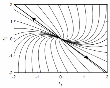
The phase portrait for this ode is shown in Fig. $\PageIndex{2}$. The dark line is the single eigenvector $\mathbf{v}$ of the matrix $\mathbf{A}$. When there is only a single eigenvector, the origin is called an improper node.