2.4: Inequalities with Absolute Value and Quadratic Functions

Last updated
Save as PDF

Page ID: 3985

$Stitz.png$
Contributed by Carl Stitz & Jeff Zeager
Professor Emeritus (Chemistry) at Lakeland Community College & Lorain County Community College

$ \newcommand{\vecs}[1]{\overset { \scriptstyle \rightharpoonup} {\mathbf{#1}} } $ $ \newcommand{\vecd}[1]{\overset{-\!-\!\rightharpoonup}{\vphantom{a}\smash {#1}}} $$\newcommand{\id}{\mathrm{id}}$ $ \newcommand{\Span}{\mathrm{span}}$ $ \newcommand{\kernel}{\mathrm{null}\,}$ $ \newcommand{\range}{\mathrm{range}\,}$ $ \newcommand{\RealPart}{\mathrm{Re}}$ $ \newcommand{\ImaginaryPart}{\mathrm{Im}}$ $ \newcommand{\Argument}{\mathrm{Arg}}$ $ \newcommand{\norm}[1]{\| #1 \|}$ $ \newcommand{\inner}[2]{\langle #1, #2 \rangle}$ $ \newcommand{\Span}{\mathrm{span}}$ $\newcommand{\id}{\mathrm{id}}$ $ \newcommand{\Span}{\mathrm{span}}$ $ \newcommand{\kernel}{\mathrm{null}\,}$ $ \newcommand{\range}{\mathrm{range}\,}$ $ \newcommand{\RealPart}{\mathrm{Re}}$ $ \newcommand{\ImaginaryPart}{\mathrm{Im}}$ $ \newcommand{\Argument}{\mathrm{Arg}}$ $ \newcommand{\norm}[1]{\| #1 \|}$ $ \newcommand{\inner}[2]{\langle #1, #2 \rangle}$ $ \newcommand{\Span}{\mathrm{span}}$

In this section, not only do we develop techniques for solving various classes of inequalities analytically, we also look at them graphically. The first example motivates the core ideas.

Example $\PageIndex{1}$:

Let $f(x) = 2x-1$ and $g(x)=5$.

Solve $f(x) = g(x)$.
Solve $f(x) < g(x)$.
Solve $f(x) > g(x)$.
Graph $y=f(x)$ and $y=g(x)$ on the same set of axes and interpret your solutions to parts 1 through 3 above.

Solution

To solve $f(x) = g(x)$, we replace $f(x)$ with $2x-1$ and $g(x)$ with $5$ to get $2x-1 = 5$. Solving for $x$, we get $x=3$.
The inequality $f(x) < g(x)$ is equivalent to $2x-1 < 5$. Solving gives $x < 3$ or $(-\infty, 3)$.
To find where $f(x) > g(x)$, we solve $2x-1 > 5$. We get $x > 3$, or $(3, \infty)$.
To graph $y=f(x)$, we graph $y = 2x-1$, which is a line with a $y$-intercept of $(0,-1)$ and a slope of $2$. The graph of $y=g(x)$ is $y=5$ which is a horizontal line through $(0,5)$.

$2.4.1a.png$

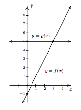
To see the connection between the graph and the Algebra, we recall the Fundamental Graphing Principle for Functions in Section 1.6: the point $(a,b)$ is on the graph of $f$ if and only if $f(a)=b$. In other words, a generic point on the graph of $y=f(x)$ is $(x,f(x))$, and a generic point on the graph of $y=g(x)$ is $(x,g(x))$. When we seek solutions to $f(x)=g(x)$, we are looking for $x$ values whose $y$ values on the graphs of $f$ and $g$ are the same. In part 1, we found $x=3$ is the solution to $f(x)=g(x)$. Sure enough, $f(3) = 5$ and $g(3) = 5$ so that the point $(3,5)$ is on both graphs. In other words, the graphs of $f$ and $g$ intersect at $(3,5)$. In part 2, we set $f(x) < g(x)$ and solved to find $x < 3$. For $x < 3$, the point $(x,f(x))$ is below $(x,g(x))$ since the $y$ values on the graph of $f$ are less than the $y$ values on the graph of $g$ there. Analogously, in part 3, we solved $f(x) > g(x)$ and found $x > 3$. For $x > 3$, note that the graph of $f$ is above the graph of $g$, since the $y$ values on the graph of $f$ are greater than the $y$ values on the graph of $g$ for those values of $x$.

$2.4.1b.png$

The preceding example demonstrates the following, which is a consequence of the Fundamental Graphing Principle for Functions.

Graphical Interpretation of Equations and Inequalities

Suppose $f$ and $g$ are functions.

The solutions to $f(x)=g(x)$ are the $x$ values where the graphs of $y=f(x)$ and $y=g(x)$ intersect.
The solution to $f(x) < g(x)$ is the set of $x$ values where the graph of $y=f(x)$ is \textit{below} the graph of $y=g(x)$.
The solution to $f(x) > g(x)$ is the set of $x$ values where the graph of $y=f(x)$ \textit{above} the graph of $y=g(x)$.

The next example turns the tables and furnishes the graphs of two functions and asks for solutions to equations and inequalities.

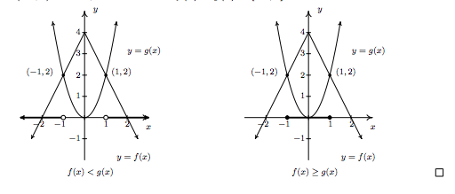
Example $\PageIndex{2}$:

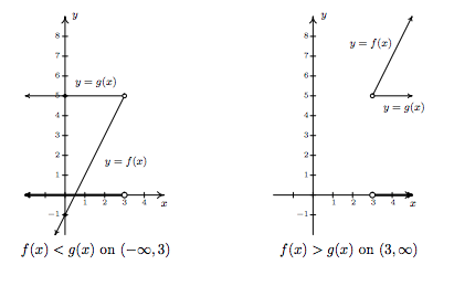
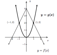
The graphs of $f$ and $g$ are below. (The graph of $y=g(x)$ is bolded.) Use these graphs to answer the following questions.

$2.4.2a.png$

Solve $f(x) = g(x)$.
Solve $f(x) < g(x)$.
Solve $f(x) \geq g(x)$.

Solution

To solve $f(x)=g(x)$, we look for where the graphs of $f$ and $g$ intersect. These appear to be at the points $(-1,2)$ and $(1,2)$, so our solutions to $f(x) = g(x)$ are $x = -1$ and $x=1$.
To solve $f(x) < g(x)$, we look for where the graph of $f$ is below the graph of $g$. This appears to happen for the $x$ values less than $-1$ and greater than $1$. Our solution is $(-\infty, -1) \cup (1,\infty)$.
To solve $f(x) \geq g(x)$, we look for solutions to $f(x)=g(x)$ as well as $f(x) > g(x)$. We solved the former equation and found $x = \pm 1$. To solve $f(x) > g(x)$, we look for where the graph of $f$ is above the graph of $g$. This appears to happen between $x=-1$ and $x=1$, on the interval $(-1,1)$. Hence, our solution to $f(x) \geq g(x)$ is $[-1,1]$.

$2.4.2b.png$

We now turn our attention to solving inequalities involving the absolute value. We have the following theorem from Intermediate Algebra to help us.

Theorem 2.4: Inequalities Involving the Absolute Value

Let $c$ be a real number. \index{inequality ! absolute value} \index{absolute value ! inequality}

For $c > 0$, $|x| < c$ is equivalent to $-c<x<c$.
For $c > 0$, $|x| \leq c$ is equivalent to $-c \leq x \leq c$.
For $c \leq 0$, $|x| < c$ has no solution, and for $c < 0$, $|x| \leq c$ has no solution.
For $c \geq 0$, $|x| > c$ is equivalent to $x<-c$ or $x>c$.
For $c \geq 0$, $|x| \geq c$ is equivalent to $x \leq -c$ or $x \geq c$.
For $c < 0$, $|x| > c$ and $|x| \geq c$ are true for all real numbers.

As with Theorem 2.1 in Section 2.2, we could argue Theorem 2.4 using cases. However, in light of what we have developed in this section, we can understand these statements graphically. For instance, if $c > 0$, the graph of $y=c$ is a horizontal line which lies above the $x$-axis through $(0,c)$. To solve $|x| < c$, we are looking for the $x$ values where the graph of $y=|x|$ is below the graph of $y=c$. We know that the graphs intersect when $|x|=c$, which, from Section 2.2, we know happens when $x=c$ or $x=-c$. Graphing, we get

$2.4a.png$

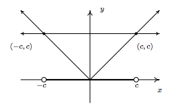
We see that the graph of $y=|x|$ is below $y=c$ for $x$ between $-c$ and $c$, and hence we get $|x| < c$ is equivalent to $-c < x < c$. The other properties in Theorem 2.4 can be shown similarly.

Example $\PageIndex{3}$:

Solve the following inequalities analytically; check your answers graphically.

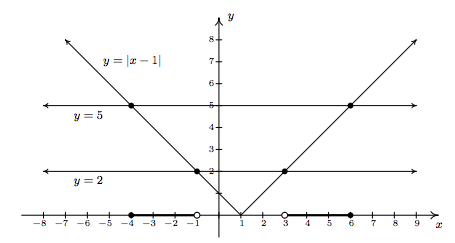
$|x-1| \geq 3$
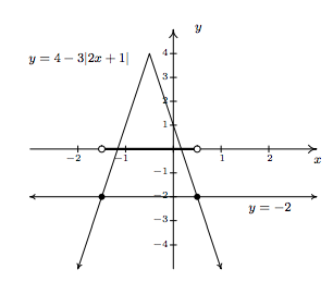
$4 - 3|2x+1| > -2$
$2 < |x-1| \leq 5$
$|x+1|\geq \dfrac{x+4}{2}$

Solution

From Theorem 2.4, $|x-1|\geq3$ is equivalent to $x-1 \leq -3$ or $x-1 \geq 3$. Solving, we get $x \leq -2$ or $x \geq 4$, which, in interval notation is $(-\infty,-2] \cup [4,\infty)$. Graphically, we have

$2.4.3a.png$

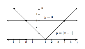
We see that the graph of $y=|x-1|$ is above the horizontal line $y=3$ for $x < -2$ and $x > 4$ hence this is where $|x-1| > 3$. The two graphs intersect when $x=-2$ and $x=4$, so we have graphical confirmation of our analytic solution.

2. To solve $4 - 3|2x+1| > -2$ analytically, we first isolate the absolute value before applying Theorem 2.4. To that end, we get $-3|2x+1|>-6$ or $|2x+1|<2$. Rewriting, we now have $-2 < 2x+1 < 2$ so that $-\frac{3}{2} < x < \frac{1}{2}$. In interval notation, we write $\left(-\frac{3}{2}, \frac{1}{2}\right)$. Graphically we see that the graph of $y=4-3|2x+1|$ is above $y=-2$ for $x$ values between $-\frac{3}{2}$ and $\frac{1}{2}$.

$2.4.3b.png$

3. Rewriting the compound inequality $2 < |x-1| \leq 5$ as `\)2 < |x-1|\) and $|x-1| \leq 5$' allows us to solve each piece using Theorem 2.4. The first inequality, $2 < |x-1|$ can be re-written as $|x-1|>2$ so $x-1 < -2$ or $x-1 > 2$. We get $x<-1$ or $x>3$. Our solution to the first inequality is then $(-\infty, -1) \cup (3, \infty)$. For $|x-1| \leq 5$, we combine results in Theorems 2.1 and 2.4 to get $-5 \leq x-1 \leq 5$ so that $-4 \leq x \leq 6$, or $[-4,6]$. Our solution to $2 < |x-1| \leq 5$ is comprised of values of $x$ which satisfy both parts of the inequality, so we take intersection\footnote{See Definition 1.2 in Section 1.1 of $(-\infty, -1) \cup (3, \infty)$ and $[-4,6]$ to get $[-4,-1) \cup (3,6]$. Graphically, we see that the graph of $y=|x-1|$ is `between' the horizontal lines $y=2$ and $y=5$ for $x$ values between $-4$ and $-1$ as well as those between $3$ and $6$. Including the $x$ values where $y=|x-1|$ and $y=5$ intersect, we get

$2.4.3c.png$

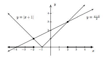
4. We need to exercise some special caution when solving $|x+1|\geq \frac{x+4}{2}$. As we saw in Example 2.2.1 in Section 2.2, when variables are both inside and outside of the absolute value, it's usually best to refer to the definition of absolute value, Definition 2.4, to remove the absolute values and proceed from there. To that end, we have $|x+1| = -(x+1)$ if $x < -1$ and $|x+1| = x+1$ if $x \geq -1$. We break the inequality into cases, the first case being when $x<-1$. For these values of $x$, our inequality becomes $-(x+1) \geq \frac{x+4}{2}$. Solving, we get $-2x-2 \geq x+4$, so that $-3x \geq 6$, which means $x \leq -2$. Since all of these solutions fall into the category $x < -1$, we keep them all. For the second case, we assume $x \geq -1$. Our inequality becomes $x+1 \geq \frac{x+4}{2}$, which gives $2x+2 \geq x+4$ or $x \geq 2$. Since all of these values of $x$ are greater than or equal to $-1$, we accept all of these solutions as well. Our final answer is $(-\infty, -2] \cup [2,\infty)$.

$2.4.3d.png$

We now turn our attention to quadratic inequalities. In the last example of Section 2.3, we needed to determine the solution to $x^2 - x -6 < 0$. We will now re-visit this problem using some of the techniques developed in this section not only to reinforce our solution in Section 2.3, but to also help formulate a general analytic procedure for solving all quadratic inequalities. If we consider $f(x) = x^2-x-6$ and $g(x)=0$, then solving $x^2 - x -6 < 0$ corresponds graphically to finding the values of $x$ for which the graph of $y=f(x)=x^2-x-6$ (the parabola) is below the graph of $y=g(x)=0$ (the $x$-axis). We've provided the graph again for reference.

$2.4b.png$

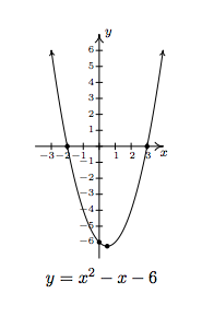
We can see that the graph of $f$ does dip below the $x$-axis between its two $x$-intercepts. The zeros of $f$ are $x=-2$ and $x=3$ in this case and they divide the domain (the $x$-axis) into three intervals: $(-\infty, -2)$, $(-2,3)$ and $(3, \infty)$. For every number in $(-\infty, -2)$, the graph of $f$ is above the $x$-axis; in other words, $f(x) > 0$ for all $x$ in $(-\infty, -2)$. Similarly, $f(x) < 0$ for all $x$ in $(-2,3)$, and $f(x) > 0$ for all $x$ in $(3, \infty)$. We can schematically represent this with the ${\bf sign diagram}$below.

$2.4c.png$

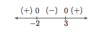
Here, the $(+)$ above a portion of the number line indicates $f(x) > 0$ for those values of $x$; the $(-)$ indicates $f(x) < 0$ there. The numbers labeled on the number line are the zeros of $f$, so we place $0$ above them. We see at once that the solution to $f(x) < 0$ is $(-2,3)$.

Our next goal is to establish a procedure by which we can generate the sign diagram without graphing the function. An important property\footnote{We will give this property a name in Chapter 3 and revisit this concept then.} of quadratic functions is that if the function is positive at one point and negative at another, the function must have at least one zero in between. Graphically, this means that a parabola can't be above the $x$-axis at one point and below the $x$-axis at another point without crossing the $x$-axis. This allows us to determine the sign of all of the function values on a given interval by testing the function at just one value in the interval. This gives us the following.

Steps for Solving a Quadratic Inequality

Rewrite the inequality, if necessary, as a quadratic function $f(x)$ on one side of the inequality and $0$ on the other.
Find the zeros of $f$ and place them on the number line with the number $0$ above them.
Choose a real number, called a \textbf{test value}, in each of the intervals determined in step 2.
Determine the sign of $f(x)$ for each test value in step 3, and write that sign above the corresponding interval.
Choose the intervals which correspond to the correct sign to solve the inequality.

Example $\PageIndex{4}$:

Solve the following inequalities analytically using sign diagrams. Verify your answer graphically.

$2x^2 \leq 3-x$
$x^2 - 2x > 1$
$x^2+1 \leq 2x$
$2x-x^2 \geq |x-1|-1$

Solution

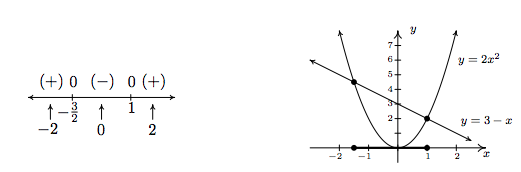
To solve $2x^2 \leq 3-x$, we first get $0$ on one side of the inequality which yields $2x^2+x-3 \leq 0$. We find the zeros of $f(x) = 2x^2 + x - 3$ by solving $2x^2 + x - 3 = 0$ for $x$. Factoring gives $(2x+3)(x-1)=0$, so $x = -\frac{3}{2}$ or $x = 1$. We place these values on the number line with $0$ above them and choose test values in the intervals $\left(-\infty, -\frac{3}{2}\right)$, $\left(-\frac{3}{2},1\right)$ and $(1,\infty)$. For the interval $\left(-\infty, -\frac{3}{2}\right)$, we choose\footnote{We have to choose $\underline{something}$ in each interval. If you don't like our choices, please feel free to choose different numbers. You'll get the same sign chart.} $x=-2$; for $\left(-\frac{3}{2},1\right)$, we pick $x=0$; and for $(1,\infty)$, $x=2$. Evaluating the function at the three test values gives us $f(-2) = 3 > 0$, so we place $(+)$ above $\left(-\infty, -\frac{3}{2}\right)$; $f(0)=-3 < 0$, so $(-)$ goes above the interval $\left(-\frac{3}{2},1\right)$; and, $f(2) = 7$, which means $(+)$ is placed above $(1,\infty)$. Since we are solving $2x^2+x-3 \leq 0$, we look for solutions to $2x^2+x-3 < 0$ as well as solutions for $2x^2+x-3 =0$. For $2x^2+x-3 < 0$, we need the intervals which we have a $(-)$. Checking the sign diagram, we see this is $\left(-\frac{3}{2},1\right)$. We know $2x^2+x-3 =0$ when $x=-\frac{3}{2}$ and $x=1$, so our final answer is $\left[-\frac{3}{2},1\right]$.

To verify our solution graphically, we refer to the original inequality, $2x^2 \leq 3-x$. We let $g(x) = 2x^2$ and $h(x)=3-x$. We are looking for the $x$ values where the graph of $g$ is below that of $h$ (the solution to $g(x) < h(x)$) as well as the points of intersection (the solutions to $g(x)=h(x)$). The graphs of $g$ and $h$ are given on the right with the sign chart on the left.

$2.4.4a.png$

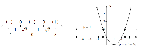
2. Once again, we re-write $x^2-2x > 1$ as $x^2-2x-1>0$ and we identify $f(x)=x^2-2x-1$. When we go to find the zeros of $f$, we find, to our chagrin, that the quadratic $x^2-2x-1$ doesn't factor nicely. Hence, we resort to the quadratic formula to solve $x^2-2x-1=0$, and arrive at $x=1 \pm \sqrt{2}$. As before, these zeros divide the number line into three pieces. To help us decide on test values, we approximate $1 - \sqrt{2} \approx -0.4$ and $1 + \sqrt{2} \approx 2.4$. We choose $x=-1$, $x=0$ and $x=3$ as our test values and find $f(-1)= 2$, which is $(+)$; $f(0)=-1$ which is $(-)$; and $f(3)=2$ which is $(+)$ again. Our solution to $x^2-2x-1>0$ is where we have $(+)$, so, in interval notation $\left(-\infty, 1-\sqrt{2}\right) \cup \left(1+\sqrt{2},\infty\right)$. To check the inequality $x^2 - 2x > 1$ graphically, we set $g(x) = x^2-2x$ and $h(x)=1$. We are looking for the $x$ values where the graph of $g$ is above the graph of $h$. As before we present the graphs on the right and the sign chart on the left.

$2.4.4b.png$

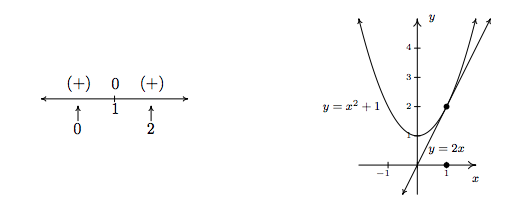
3. To solve $x^2+1 \leq 2x$, as before, we solve $x^2-2x+1 \leq 0$. Setting $f(x) = x^2-2x+1=0$, we find the only one zero of $f$, $x = 1$. This one $x$ value divides the number line into two intervals, from which we choose $x=0$ and $x=2$ as test values. We find $f(0)=1 > 0$ and $f(2) = 1 > 0$. Since we are looking for solutions to $x^2-2x+1 \leq 0$, we are looking for $x$ values where $x^2-2x+1 < 0$ as well as where $x^2-2x+1 = 0$. Looking at our sign diagram, there are no places where $x^2-2x+1 < 0$ (there are no $(-)$), so our solution is only $x=1$ (where $x^2-2x+1 = 0$). We write this as $\left\{1\right\}$. Graphically, we solve $x^2+1 \leq 2x$ by graphing $g(x) = x^2+1$ and $h(x)=2x$. We are looking for the $x$ values where the graph of $g$ is below the graph of $h$ (for $x^2+1 < 2x$) and where the two graphs intersect (\)x^2+1 = 2x\)). Notice that the line and the parabola touch at $\left(1, 2\right)$, but the parabola is always above the line otherwise.\footnote{In this case, we say the line $y=2x$ is $\textbf{tangent}$ to $y=x^2+1$ at $\left(1, 2\right)$. Finding tangent lines to arbitrary functions is a fundamental problem solved, in general, with Calculus.}

$2.4.4c.png$

4. To solve our last inequality, $2x-x^2 \geq |x-1|-1$, we re-write the absolute value using cases. For $x < 1$, $|x-1| = -(x-1) = 1-x$, so we get $2x-x^2 \geq 1-x-1$, or $x^2-3x \leq 0$. Finding the zeros of $f(x) = x^2-3x$, we get $x=0$ and $x=3$. However, we are only concerned with the portion of the number line where $x < 1$, so the only zero that we concern ourselves with is $x=0$. This divides the interval $x<1$ into two intervals: $(-\infty, 0)$ and $(0,1)$. We choose $x=-1$ and $x=\frac{1}{2}$ as our test values. We find $f(-1) = 4$ and $f\left(\frac{1}{2}\right) = -\frac{5}{4}$. Hence, our solution to $x^2-3x \leq 0$ for $x < 1$ is $[0,1)$. Next, we turn our attention to the case $x \geq 1$. Here, $|x-1| = x-1$, so our original inequality becomes $2x-x^2 \geq x-1-1$, or $x^2-x-2 \leq 0$. Setting $g(x) = x^2-x-2$, we find the zeros of $g$ to be $x=-1$ and $x=2$. Of these, only $x=2$ lies in the region $x \geq 1$, so we ignore $x=-1$. Our test intervals are now $[1,2)$ and $(2,\infty)$. We choose $x=1$ and $x=3$ as our test values and find $g(1) = -2$ and $g(3) = 4$. Hence, our solution to $g(x) = x^2-x-2 \leq 0$, in this region is $[1,2)$.

$2.4.4d.png$

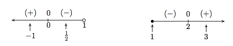
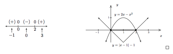
Combining these into one sign diagram, we have that our solution is $[0,2]$. Graphically, to check $2x-x^2 \geq |x-1|-1$, we set $h(x) = 2x-x^2$ and $i(x) = |x-1|-1$ and look for the $x$ values where the graph of $h$ is above the the graph of $i$ (the solution of $h(x) > i(x)$) as well as the $x$-coordinates of the intersection points of both graphs (where $h(x)=i(x)$). The combined sign chart is given on the left and the graphs are on the right.

$2.4.4e.png$

One of the classic applications of inequalities is the notion of tolerances.\footnote{The underlying concept of Calculus can be phrased in terms of tolerances, so this is well worth your attention.} Recall that for real numbers $x$ and $c$, the quantity $|x-c|$ may be interpreted as the distance from $x$ to $c$. Solving inequalities of the form $|x-c| \leq d$ for $d \geq 0$ can then be interpreted as finding all numbers $x$ which lie within $d$ units of $c$. We can think of the number $d$ as a `tolerance' and our solutions $x$ as being within an accepted tolerance of $c$. We use this principle in the next example.

Example $\PageIndex{5}$:

The area $A$ (in square inches) of a square piece of particle board which measures $x$ inches on each side is $A(x) = x^2$. Suppose a manufacturer needs to produce a $24$ inch by $24$ inch square piece of particle board as part of a home office desk kit. How close does the side of the piece of particle board need to be cut to $24$ inches to guarantee that the area of the piece is within a tolerance of $0.25$ square inches of the target area of $576$ square inches?

Solution

Mathematically, we express the desire for the area $A(x)$ to be within $0.25$ square inches of $576$ as $|A - 576| \leq 0.25$. Since $A(x) = x^2$, we get $|x^2 - 576| \leq 0.25$, which is equivalent to $-0.25 \leq x^2 - 576 \leq 0.25$. One way to proceed at this point is to solve the two inequalities $-0.25 \leq x^2 - 576$ and $x^2 - 576 \leq 0.25$ individually using sign diagrams and then taking the intersection of the solution sets. While this way will (eventually) lead to the correct answer, we take this opportunity to showcase the increasing property of the square root: if $0 \leq a \leq b$, then $\sqrt{a} \leq \sqrt{b}$. To use this property, we proceed as follows

\[ \begin{array}{rclr} -0.25 \leq & x^2 - 576 & \leq 0.25 & \\ 575.75 \leq & x^2 & \leq 576.25 & \text{(add $576$ across the inequalities.)} \\ \sqrt{575.75} \leq & \sqrt{x^2} & \leq \sqrt{576.25} & \text{(take square roots.)} \\ \sqrt{575.75} \leq & |x| & \leq \sqrt{576.25} & \text{(\)\sqrt{x^2} = |x|\))} \\ \end{array} \]

By Theorem 2.4, we find the solution to $\sqrt{575.75} \leq |x|$ to be $\left(-\infty, -\sqrt{575.75} \, \right] \cup \left[\sqrt{575.75}, \infty \right)$ and the solution to $|x| \leq \sqrt{576.25}$ to be $\left[-\sqrt{576.25}, \sqrt{576.25} \, \right]$. To solve $\sqrt{575.75} \leq |x| \leq \sqrt{576.25}$, we intersect these two sets to get $[-\sqrt{576.25}, -\sqrt{575.75}] \cup [\sqrt{575.75},\sqrt{576.25}]$. Since $x$ represents a length, we discard the negative answers and get $[\sqrt{575.75},\sqrt{576.25}]$. This means that the side of the piece of particle board must be cut between $\sqrt{575.75} \approx 23.995$ and $\sqrt{576.25} \approx 24.005$ inches, a tolerance of (approximately) $0.005$ inches of the target length of $24$ inches.

Our last example in the section demonstrates how inequalities can be used to describe regions in the plane, as we saw earlier in Section 1.2.

Example $\PageIndex{6}$:

Sketch the following relations.

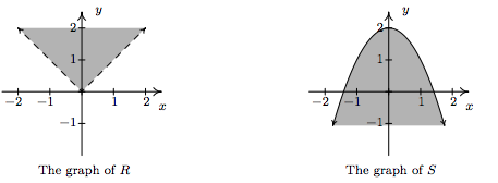
$R = \{ (x,y) : y > |x| \}$
$S = \{ (x,y) : y \leq 2-x^2 \}$
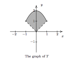
$T = \{ (x,y) : |x| < y \leq 2-x^2 \}$

Solution

The relation $R$ consists of all points $(x,y)$ whose $y$-coordinate is greater than $|x|$. If we graph $y=|x|$, then we want all of the points in the plane above the points on the graph. Dotting the graph of $y=|x|$ as we have done before to indicate that the points on the graph itself are not in the relation, we get the shaded region below on the left.
For a point to be in $S$, its $y$-coordinate must be less than or equal to the $y$-coordinate on the parabola $y=2-x^2$. This is the set of all points below or on the parabola $y=2-x^2$.

$2.4.6a.png$

3. Finally, the relation $T$ takes the points whose $y$-coordinates satisfy both the conditions given in $R$ and those of $S$. Thus we shade the region between $y=|x|$ and $y=2-x^2$, keeping those points on the parabola, but not the points on $y=|x|$. To get an accurate graph, we need to find where these two graphs intersect, so we set $|x| = 2-x^2$. Proceeding as before, breaking this equation into cases, we get $x=-1,1$. Graphing yields

$2.4.6b.png$

Contributors and Attributions

Carl Stitz, Ph.D. (Lakeland Community College) and Jeff Zeager, Ph.D. (Lorain County Community College)