5.3: Inverse Functions

Thinking of a function as a process like we did in Section 1.4, in this section we seek another function which might reverse that process. As in real life, we will find that some processes (like putting on socks and shoes) are reversible while some (like cooking a steak) are not. We start by discussing a very basic function which is reversible, \(f(x) = 3x+4\). Thinking of \(f\) as a process, we start with an input \(x\) and apply two steps, as we saw in Section 1.4

1. multiply by \(3\)
2. add \(4\)

To reverse this process, we seek a function \(g\) which will undo each of these steps and take the output from \(f\), \(3x+4\), and return the input \(x\). If we think of the real-world reversible two-step process of first putting on socks then putting on shoes, to reverse the process, we first take off the shoes, and then we take off the socks. In much the same way, the function \(g\) should undo the second step of \(f\) first. That is, the function \(g\) should

1. subtract \(4\)
2. divide by \(3\)

Following this procedure, we get \(g(x) = \frac{x-4}{3}\). Let's check to see if the function \(g\) does the job. If \(x=5\), then \(f(5) = 3(5)+4 = 15+4 = 19\). Taking the output \(19\) from \(f\), we substitute it into \(g\) to get \(g(19) = \frac{19-4}{3} = \frac{15}{3} = 5\), which is our original input to \(f\). To check that \(g\) does the job for all \(x\) in the domain of \(f\), we take the generic output from \(f\), \(f(x) = 3x+4\), and substitute that into \(g\). That is, \(g(f(x)) = g(3x+4) = \frac{(3x+4)-4}{3} = \frac{3x}{3} = x\), which is our original input to \(f\). If we carefully examine the arithmetic as we simplify \(g(f(x))\), we actually see \(g\) first `undoing' the addition of \(4\), and then `undoing' the multiplication by \(3\). Not only does \(g\) undo \(f\), but \(f\) also undoes \(g\). That is, if we take the output from \(g\), \(g(x) = \frac{x-4}{3}\), and put that into \(f\), we get \(f(g(x)) = f\left(\frac{x-4}{3}\right) = 3 \left(\frac{x-4}{3}\right) + 4 = (x-4) + 4 = x\). Using the language of function composition developed in Section 5.1, the statements \(g(f(x)) = x\) and \(f(g(x)) = x\) can be written as \((g \circ f)(x) = x\) and \((f \circ g)(x) = x\), respectively. Abstractly, we can visualize the relationship between \(f\) and \(g\) in the diagram below.

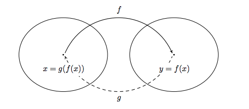
The main idea to get from the diagram is that \(g\) takes the outputs from \(f\) and returns them to their respective inputs, and conversely, \(f\) takes outputs from \(g\) and returns them to their respective inputs. We now have enough background to state the central definition of the section.

Definition 5.2 :

Suppose \(f\) and \(g\) are two functions such that

1. \((g \circ f)(x) = x\) for all \(x\) in the domain of \(f\) \(\textbf{and}\)
2. \((f \circ g)(x) = x\) for all \(x\) in the domain of \(g\)

then \(f\) and \(g\) are said to be inverses of each other. The functions \(f\) and \(g\) are said to be invertible.

We now formalize the concept that inverse functions exchange inputs and outputs.

Theorem 5.2: Properties of Inverse Functions

Suppose \(f\) and \(g\) are inverse functions.

1. The range (i..e, the set of all outputs of a function) of \(f\) is the domain of \(g\) and the domain of \(f\) is the range of \(g\)
2. \(f(a) = b\) if and only if \(g(b) = a\)
3. \((a,b)\) is on the graph of \(f\) if and only if \((b,a)\) is on the graph of \(g\)

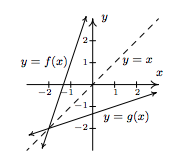
Theorem 5.2 is a consequence of Definition 5.2 and the Fundamental Graphing Principle for Functions. We note the third property in Theorem 5.2 tells us that the graphs of inverse functions are reflections about the line \(y=x\). For a proof of this, see Example 1.1.7 in Section 1.1 and Exercise 72 in Section 2.1. For example, we plot the inverse functions \(f(x) = 3x+4\) and \(g(x) = \frac{x-4}{3}\) below.

If we abstract one step further, we can express the sentiment in Definition 5.2 by saying that \(f\) and \(g\) are inverses if and only if \(g \circ f = I_{1}\) and \(f \circ g = I_{2}\) where \(I_{1}\) is the identity function restricted \footnote{The identity function \(I\), which was introduced in Section 2.1 and mentioned in Theorem 5.1, has a domain of all real numbers. Since the domains of \(f\) and \(g\) may not be all real numbers, we need the restrictions listed here.} to the domain of \(f\) and \(I_{2}\) is the identity function restricted to the domain of \(g\). In other words, \(I_{1}(x) = x\) for all \(x\) in the domain of \(f\) and \(I_{2}(x) = x\) for all \(x\) in the domain of \(g\). Using this description of inverses along with the properties of function composition listed in Theorem 5.1, we can show that function inverses are unique.\footnote{In other words, invertible functions have exactly one inverse.} Suppose \(g\) and \(h\) are both inverses of a function \(f\). By Theorem 5.2, the domain of \(g\) is equal to the domain of \(h\), since both are the range of \(f\). This means the identity function \(I_{2}\) applies both to the domain of \(h\) and the domain of \(g\). Thus \(h = h \circ I_{2} = h \circ (f \circ g) = (h \circ f) \circ g = I_{1} \circ g = g\), as required.\footnote{It is an excellent exercise to explain each step in this string of equalities.} We summarize the discussion of the last two paragraphs in the following theorem. \footnote{In the interests of full disclosure, the authors would like to admit that much of the discussion in the previous paragraphs could have easily been avoided had we appealed to the description of a function as a set of ordered pairs. We make no apology for our discussion from a function composition standpoint, however, since it exposes the reader to more abstract ways of thinking of functions and inverses. We will revisit this concept again in Chapter 8.}

THEOREM 5.3: Uniqueness of Inverse Functions and Their Graphs

Suppose \(f\) is an invertible function.

• There is exactly one inverse function for \(f\), denoted \(f^{-1}\) (read \(f\)-inverse)
• The graph of \(y=f^{-1}(x)\) is the reflection of the graph of \(y=f(x)\) across the line \(y=x\).

The notation \(f^{-1}\) is an unfortunate choice since you've been programmed since Elementary Algebra to think of this as \(\frac{1}{f}\). This is most definitely \(\textit{not}\) the case since, for instance, \(f(x) = 3x+4\) has as its inverse \(f^{-1}(x) = \frac{x-4}{3}\), which is certainly different than \(\frac{1}{f(x)} = \frac{1}{3x+4}\). Why does this confusing notation persist? As we mentioned in Section 5.1, the identity function \(I\) is to function composition what the real number \(1\) is to real number multiplication. The choice of notation \(f^{-1}\) alludes to the property that \(f^{-1} \circ f = I_{1}\) and \(f \circ f^{-1} = I_{2}\), in much the same way as \(3^{-1} \cdot 3 = 1\) and \(3 \cdot 3^{-1} = 1\).

Let's turn our attention to the function \(f(x) = x^2\). Is \(f\) invertible? A likely candidate for the inverse is the function \(g(x) = \sqrt{x}\). Checking the composition yields \((g\circ f)(x) = g(f(x)) = \sqrt{x^2} = |x|\), which is not equal to \(x\) for all \(x\) in the domain \((-\infty, \infty)\). For example, when \(x=-2\), \(f(-2)= (-2)^2 = 4\), but \(g(4) = \sqrt{4}=2\), which means \(g\) failed to return the input \(-2\) from its output \(4\). What \(g\) did, however, is match the output \(4\) to a \(\textit{different}\) input, namely \(2\), which satisfies \(f(2) = 4\). This issue is presented schematically in the picture below.

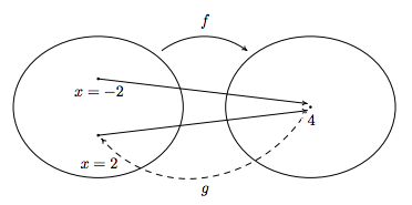
We see from the diagram that since both \(f(-2)\) and \(f(2)\) are \(4\), it is impossible to construct a \(\textit{function}\) which takes \(4\) back to \(\textit{both}\) \(x=2\) and \(x=-2\). (By definition, a function matches a real number with exactly one other real number.) From a graphical standpoint, we know that if \(y=f^{-1}(x)\) exists, its graph can be obtained by reflecting \(y=x^2\) about the line \(y=x\), in accordance with Theorem 5.3. Doing so produces

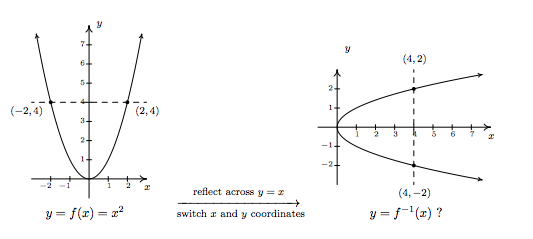
We see that the line \(x=4\) intersects the graph of the supposed inverse twice - meaning the graph fails the Vertical Line Test, Theorem 1.1, and as such, does not represent \(y\) as a function of \(x\). The vertical line \(x=4\) on the graph on the right corresponds to the \(\textit{horizontal line\)} \(y=4\) on the graph of \(y=f(x)\). The fact that the horizontal line \(y=4\) intersects the graph of \(f\) twice means two \(\textit{different}\) inputs, namely \(x=-2\) and \(x=2\), are matched with the \(\textit{same}\) output, \(4\), which is the cause of all of the trouble. In general, for a function to have an inverse, \(\textit{different}\) inputs must go to \(\textit{different}\) outputs, or else we will run into the same problem we did with \(f(x) = x^2\). We give this property a name.

Definition 5.3: One-to-One Functions

A function \(f\) is said to be one-to-one if \(f\) matches different inputs to different outputs. Equivalently, \(f\) is one-to-one if and only if whenever \(f(c) = f(d)\), then \(c=d\). \index{one-to-one function}

Graphically, we detect one-to-one functions using the test below.

Theorem 5.4: The Horizontal Line Test

A function \(f\) is one-to-one if and only if no horizontal line intersects the graph of \(f\) more than once.

We say that the graph of a function \(\textbf{passes}\) the Horizontal Line Test if no horizontal line intersects the graph more than once; otherwise, we say the graph of the function \(\textbf{fails}\) the Horizontal Line Test. We have argued that if \(f\) is invertible, then \(f\) must be one-to-one, otherwise the graph given by reflecting the graph of \(y = f(x)\) about the line \(y = x\) will fail the Vertical Line Test. It turns out that being one-to-one is also enough to guarantee invertibility. To see this, we think of \(f\) as the set of ordered pairs which constitute its graph. If switching the \(x\)- and \(y\)-coordinates of the points results in a function, then \(f\) is invertible and we have found \(f^{-1}\). This is precisely what the Horizontal Line Test does for us: it checks to see whether or not a set of points describes \(x\) as a function of \(y\). We summarize these results below.

Theorem 5.5: Equivalent Conditions for Invertibility

Suppose \(f\) is a function. The following statements are equivalent. \index{invertibility ! function}

• \(f\) is invertible
• \(f\) is one-to-one
• The graph of \(f\) passes the Horizontal Line Test

We put this result to work in the next example.

Example \(\PageIndex{1}\):inversefunctiononetooneex

Determine if the following functions are one-to-one in two ways: (a) analytically using Definition 5.3 and (b) graphically using the Horizontal Line Test.

1. \(f(x) = \dfrac{1-2x}{5}\)
2. \(g(x) = \dfrac{2x}{1-x}\)
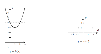
3. \(h(x) = x^2 - 2x+4\)
4. \(F = \{(-1,1), (0,2), (2,1)\}\)

Solution

1. (a) To determine if \(f\) is one-to-one analytically, we assume \(f(c) = f(d)\) and attempt to deduce that \(c=d\).

\[ \begin{array}{rclr} f(c) & = & f(d) & \\ \dfrac{1-2c}{5} & = & \dfrac{1-2d}{5} & \\ 1-2c & = & 1-2d & \\ -2c & = & -2d & \\ c & = & d \, \, \checkmark & \\ \end{array} \]

Hence, \(f\) is one-to-one.

(b) To check if \(f\) is one-to-one graphically, we look to see if the graph of \(y=f(x)\) passes the Horizontal Line Test. We have that \(f\) is a non-constant linear function, which means its graph is a non-horizontal line. Thus the graph of \(f\) passes the Horizontal Line Test.

2 (a) We begin with the assumption that \(g(c) = g(d)\) and try to show \(c=d\).

\[ \begin{array}{rclr} g(c) & = & g(d) & \\ \dfrac{2c}{1-c} & = & \dfrac{2d}{1-d} & \\ 2c(1-d) & = & 2d(1-c) & \\ 2c - 2cd & = & 2d - 2dc & \\ 2c & = & 2d & \\ c & = & d \, \, \checkmark \\ \end{array} \]

We have shown that \(g\) is one-to-one.

(b) We can graph \(g\) using the six step procedure outlined in Section 4.2. We get the sole intercept at \((0,0)\), a vertical asymptote \(x=1\) and a horizontal asymptote (which the graph never crosses) \(y = -2\). We see from that the graph of \(g\) passes the Horizontal Line Test.

3. (a) We begin with \(h(c) = h(d)\). As we work our way through the problem, we encounter a nonlinear equation. We move the non-zero terms to the left, leave a \(0\) on the right and factor accordingly.

\[ \begin{array}{rclr} h(c) & = & h(d) & \\ c^2 - 2c+4 & = & d^2 - 2d+4 & \\ c^2 - 2c & = & d^2 - 2d & \\ c^2 - d^2 - 2c + 2d & = & 0 & \\ (c+d)(c-d) - 2(c-d) & = & 0 & \\ (c-d)((c+d) -2) & = & 0 & \mbox{factor by grouping} \\ c-d = 0 & \mbox{or} & c+d -2 = 0 & \\ c = d & \mbox{or} & c = 2-d & \\ \end{array} \]

We get \(c=d\) as one possibility, but we also get the possibility that \(c=2-d\). This suggests that \(f\) may not be one-to-one. Taking \(d=0\), we get \(c = 0\) or \(c = 2\). With \(f(0) = 4\) and \(f(2) = 4\), we have produced two different inputs with the same output meaning \(f\) is not one-to-one.

(b) We note that \(h\) is a quadratic function and we graph \(y=h(x)\) using the techniques presented in Section 2.3. The vertex is \((1,3)\) and the parabola opens upwards. We see immediately from the graph that \(h\) is not one-to-one, since there are several horizontal lines which cross the graph more than once.

4. (a) The function \(F\) is given to us as a set of ordered pairs. The condition \(F(c)=F(d)\) means the outputs from the function (the \(y\)-coordinates of the ordered pairs) are the same. We see that the points \((-1,1)\) and \((2,1)\) are both elements of \(F\) with \(F(-1)=1\) and \(F(2) = 1\). Since \(-1 \neq 2\), we have established that \(F\) is \(\textit{not}\) one-to-one.

(b) Graphically, we see the horizontal line \(y=1\) crosses the graph more than once. Hence, the graph of \(F\) fails the Horizontal Line Test.

We have shown that the functions \(f\) and \(g\) in Example 5.2.1 are one-to-one. This means they are invertible, so it is natural to wonder what \(f^{-1}(x)\) and \(g^{-1}(x)\) would be. For \(f(x) = \frac{1-2x}{5}\), we can think our way through the inverse since there is only one occurrence of \(x\). We can track step-by-step what is done to \(x\) and reverse those steps as we did at the beginning of the chapter. The function \(g(x) = \frac{2x}{1-x}\) is a bit trickier since \(x\) occurs in two places. When one evaluates \(g(x)\) for a specific value of \(x\), which is first, the \(2x\) or the \(1-x\)? We can imagine functions more complicated than these so we need to develop a general methodology to attack this problem. Theorem 5.2 tells us equation \(y = f^{-1}(x)\) is equivalent to \(f(y) = x\) and this is the basis of our algorithm.

Steps for finding the Inverse of a One-to-one Function

1. Write \(y=f(x)\)
2. Interchange \(x\) and \(y\)
3. Solve \(x = f(y)\) for \(y\) to obtain \(y=f^{-1}(x)\)

Note that we could have simply written `Solve \(x=f(y)\) for \(y\)' and be done with it. The act of interchanging the \(x\) and \(y\) is there to remind us that we are finding the inverse function by switching the inputs and outputs.

Example \(\PageIndex{2}\):

Find the inverse of the following one-to-one functions. Check your answers analytically using function composition and graphically.

1. \(f(x) = \dfrac{1-2x}{5}\)
2. \(g(x) = \dfrac{2x}{1-x}\)

Solution

1. As we mentioned earlier, it is possible to think our way through the inverse of \(f\) by recording the steps we apply to \(x\) and the order in which we apply them and then reversing those steps in the reverse order. We encourage the reader to do this. We, on the other hand, will practice the algorithm. We write \(y=f(x)\) and proceed to switch \(x\) and \(y\)

\[ \begin{array}{rclr} y & = & f(x) & \\ y & = & \dfrac{1-2x}{5} & \\ x & = & \dfrac{1-2y}{5} & \mbox{switch \(x\) and \(y\)} \\ 5x & = & 1 - 2y & \\ 5x-1 & = & -2y & \\ \dfrac{5x-1}{-2} & = & y & \\ y & = & -\dfrac{5}{2} x + \dfrac{1}{2} & \\ \end{array} \]

We have \(f^{-1}(x) = -\frac{5}{2} x + \frac{1}{2}\). To check this answer analytically, we first check that \(\left(f^{-1} \circ f \right)(x) = x \) for all \(x\) in the domain of \(f\), which is all real numbers.

\[ \begin{array}{rclr} \left(f^{-1} \circ f \right)(x) & = & f^{-1}(f(x)) & \\ & = & -\dfrac{5}{2} f(x) + \dfrac{1}{2} & \\ & = & -\dfrac{5}{2} \left(\dfrac{1-2x}{5}\right) + \dfrac{1}{2} & \\ & = & -\dfrac{1}{2} (1-2x) + \dfrac{1}{2} & \\ & = & -\dfrac{1}{2} + x + \dfrac{1}{2} & \\ & = & x \, \, \checkmark \\ \end{array}\]

We now check that \(\left(f \circ f^{-1} \right)(x) = x \) for all \(x\) in the range of \(f\) which is also all real numbers. (Recall that the domain of \(f^{-1}\)) is the range of \(f\).)

\[ \begin{array}{rclr} \left(f \circ f^{-1} \right)(x) & = & f(f^{-1}(x)) & \\ & = &\dfrac{1-2f^{-1}(x)}{5} & \\ & = &\dfrac{1-2\left( -\frac{5}{2} x + \frac{1}{2} \right)}{5} & \\ & = & \dfrac{1+5x-1}{5} & \\ & = &\dfrac{5x}{5} & \\ & = & x \, \, \checkmark\\ \end{array}\]

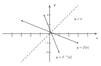
To check our answer graphically, we graph \(y=f(x)\) and \(y=f^{-1}(x)\) on the same set of axes.\footnote{Note that if you perform your check on a calculator for more sophisticated functions, you'll need to take advantage of the `ZoomSquare' feature to get the correct geometric perspective.} They appear to be reflections across the line \(y=x\).

2. To find \(g^{-1}(x)\), we start with \(y=g(x)\). We note that the domain of \(g\) is \((-\infty,1) \cup (1, \infty)\).

\[ \begin{array}{rclr} y & = & g(x) & \\ y & = & \dfrac{2x}{1-x} & \\ x & = & \dfrac{2y}{1-y} & \mbox{switch \(x\) and \(y\)} \\ x(1-y) & = & 2y & \\ x-xy & = & 2y & \\ x & = & xy + 2y & \\ x & = & y(x+2) & \mbox{factor}\\ [8pt] y & = & \dfrac{x}{x+2} \end{array} \]

We obtain \(g^{-1}(x) = \frac{x}{x+2}\). To check this analytically, we first check \(\left(g^{-1} \circ g \right)(x) = x\) for all \(x\) in the domain of \(g\), that is, for all \(x \neq 1\).

Next, we check \(g\left(g^{-1}(x)\right)= x\) for all \(x\) in the range of \(g\). From the graph of \(g\) in Example 5.2.1, we have that the range of \(g\) is \((-\infty, -2) \cup (-2,\infty)\). This matches the domain we get from the formula \(g^{-1}(x) = \frac{x}{x+2}\), as it should.

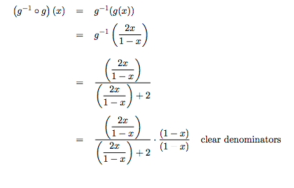
\[ \begin{array}{rclr} \left(g \circ g^{-1} \right)(x) & = & g\left(g^{-1}(x)\right) & \\ & = & g \left(\dfrac{x}{x+2}\right) & \\ & = & \dfrac{ 2\left(\dfrac{x}{x+2}\right)}{ 1-\left(\dfrac{x}{x+2}\right)} \\ & = & \dfrac{ 2\left(\dfrac{x}{x+2}\right)}{ 1-\left(\dfrac{x}{x+2}\right)} \cdot \dfrac{(x+2)}{(x+2)} & \mbox{clear denominators} \\ & = & \dfrac{ 2x}{ (x+2) -x} & \\ & = & \dfrac{2x}{2} & \\ & = & x \, \, \checkmark \\ \end{array} \]

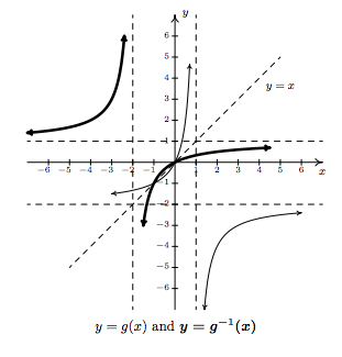
Graphing \(y=g(x)\) and \(y = g^{-1}(x)\) on the same set of axes is busy, but we can see the symmetric relationship if we thicken the curve for \(y=g^{-1}(x)\). Note that the vertical asymptote \(x=1\) of the graph of \(g\) corresponds to the horizontal asymptote \(y=1\) of the graph of \(g^{-1}\), as it should since \(x\) and \(y\) are switched. Similarly, the horizontal asymptote \(y=-2\) of the graph of \(g\) corresponds to the vertical asymptote \(x=-2\) of the graph of \(g^{-1}\).

We now return to \(f(x) = x^2\). We know that \(f\) is not one-to-one, and thus, is not invertible. However, if we restrict the domain of \(f\), we can produce a new function \(g\) which is one-to-one. If we define \(g(x) = x^2\), \(x \geq 0\), then we have

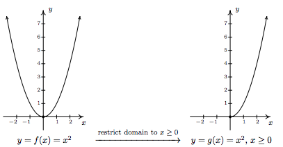
The graph of \(g\) passes the Horizontal Line Test. To find an inverse of \(g\), we proceed as usual

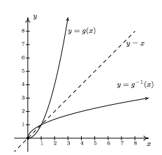
\[ \begin{array}{rclr} y & = & g(x) & \\ y & = & x^2, \, \, \, x \geq 0 & \\ x & = & y^2, \, \, \, y \geq 0 & \mbox{switch \(x\) and \(y\)}\\ y & = & \pm \sqrt{x} & \\ y & = & \sqrt{x} & \mbox{since \(y \geq 0\)} \\ \end{array} \]

We get \(g^{-1}(x) = \sqrt{x}\). At first it looks like we'll run into the same trouble as before, but when we check the composition, the domain restriction on \(g\) saves the day. We get \(\left(g^{-1} \circ g\right) (x) = g^{-1}(g(x)) = g^{-1}\left(x^2\right) = \sqrt{x^2} = |x| = x\), since \(x \geq 0\). Checking \(\left( g \circ g^{-1}\right)(x) = g\left(g^{-1}(x)\right) = g\left(\sqrt{x}\right) = \left(\sqrt{x}\right)^2 = x\). Graphing\footnote{We graphed \(y=\sqrt{x}\) in Section 1.7.} \(g\) and \(g^{-1}\) on the same set of axes shows that they are reflections about the line \(y=x\).

Our next example continues the theme of domain restriction.

Example \(\PageIndex{3}\):inverserestrictionex

Graph the following functions to show they are one-to-one and find their inverses. Check your answers analytically using function composition and graphically.

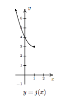
1. \(j(x) = x^2 - 2x + 4\), \(x \leq 1\).
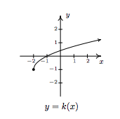
2. \(k(x) = \sqrt{x+2} - 1\)

Solution

1. The function \(j\) is a restriction of the function \(h\) from Example 5.2.1. Since the domain of \(j\) is restricted to \(x \leq 1\), we are selecting only the `left half' of the parabola. We see that the graph of \(j\) passes the Horizontal Line Test and thus \(j\) is invertible.

We now use our algorithm \footnote{Here, we use the Quadratic Formula to solve for \(y\). For `completeness,' we note you can (and should!) also consider solving for \(y\) by `completing' the square.} to find \(j^{-1}(x)\).

\[ \begin{array}{rclr} y & = & j(x) & \\ y & = & x^2-2x+4, \, \, \, x \leq 1 \\ x & = & y^2 - 2y+4, \, \, \, y \leq 1 & \mbox{switch \(x\) and \(y\)} \\ 0 & = & y^2 - 2y + 4-x & \\ y & = & \dfrac{2 \pm \sqrt{(-2)^2-4(1)(4-x)}}{2(1)} & \mbox{quadratic formula, \(c=4-x\)} \\ [10pt] y & = & \dfrac{2 \pm \sqrt{4x-12}}{2} & \\ y & = & \dfrac{2 \pm \sqrt{4(x-3)}}{2} & \\ y & = & \dfrac{2 \pm 2\sqrt{x-3}}{2} & \\ y & = & \dfrac{2\left(1 \pm \sqrt{x-3}\right)}{2} & \\ y & = & 1 \pm \sqrt{x-3} & \\ y & = & 1 - \sqrt{x-3} & \mbox{since \(y \leq 1\).} \\ \end{array}\]

We have \(j^{-1}(x) = 1 - \sqrt{x-3}\). When we simplify \(\left(j^{-1} \circ j\right)(x)\), we need to remember that the domain of \(j\) is \(x \leq 1\).

\[ \begin{array}{rclr} \left(j^{-1} \circ j \right)(x) & = & j^{-1}(j(x)) & \\ & = & j^{-1}\left(x^2-2x+4\right), \, \, \, x \leq 1 & \\ & = & 1 - \sqrt{\left(x^2-2x+4\right)-3} & \\ & = & 1 - \sqrt{x^2-2x+1} & \\ & = & 1 - \sqrt{(x-1)^2} & \\ & = & 1 - |x-1|& \\ & = & 1 - (-(x-1)) & \mbox{since \(x \leq 1\)}\\ & = & x \, \, \checkmark &\\ \end{array}\]

Checking \(j \circ j^{-1}\), we get

\[ \begin{array}{rclr} \left(j \circ j^{-1} \right)(x) & = & j\left(j^{-1}(x)\right) & \\ & = & j\left(1 - \sqrt{x-3}\right) & \\ & = & \left(1 - \sqrt{x-3}\right)^2-2\left(1 - \sqrt{x-3}\right)+4 & \\ & = & 1 - 2\sqrt{x-3} + \left(\sqrt{x-3}\right)^2 -2 + 2\sqrt{x-3}+4 & \\ & = & 3+ x-3 & \\ & = & x \, \, \checkmark &\\ \end{array}\]

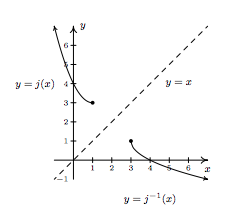
Using what we know from Section 1.7, we graph \(y=j^{-1}(x)\) and \(y=j(x)\) below.

2. We graph \(y=k(x) =\sqrt{x+2} - 1\) using what we learned in Section 1.7 and see \(k\) is one-to-one.

We now try to find \(k^{-1}\).

\[ \begin{array}{rclr} y & = & k(x) & \\ y & = & \sqrt{x+2}-1 & \\ x & = & \sqrt{y+2} - 1 & \mbox{switch \(x\) and \(y\)} \\ x+1 & = & \sqrt{y+2} & \\ (x+1)^2 & = & \left(\sqrt{y+2}\right)^2 & \\ x^2 + 2x + 1 & = & y + 2 & \\ y & = & x^2 + 2x - 1 & \\ \end{array} \]

We have \(k^{-1}(x) = x^2+2x-1\). Based on our experience, we know something isn't quite right. We determined \(k^{-1}\) is a quadratic function, and we have seen several times in this section that these are not one-to-one unless their domains are suitably restricted. Theorem 5.2 tells us that the domain of \(k^{-1}\) is the range of \(k\). From the graph of \(k\), we see that the range is \([-1, \infty)\), which means we restrict the domain of \(k^{-1}\) to \(x \geq -1\). We now check that this works in our compositions.

\[ \begin{array}{rclr} \left(k^{-1} \circ k \right)(x) & = & k^{-1}(k(x)) & \\ & = & k^{-1}\left(\sqrt{x+2}-1\right), \, \, \, x \geq -2 & \\ & = & \left(\sqrt{x+2}-1\right)^2 + 2\left(\sqrt{x+2}-1\right) - 1& \\ & = & \left(\sqrt{x+2}\right)^2 - 2\sqrt{x+2} + 1 + 2 \sqrt{x+2} - 2 - 1 & \\ & = &x+2 -2 & \\ & = & x \, \, \checkmark &\\ \end{array}\]

and

\[ \begin{array}{rclr} \left(k \circ k^{-1} \right)(x) & = & k\left( x^2+2x-1 \right) \, \, \, x \geq -1 & \\ & = & \sqrt{\left(x^2+2x-1\right)+2}-1 & \\ & = & \sqrt{x^2+2x+1}-1 & \\ & = & \sqrt{(x+1)^2}-1 & \\ & = & |x+1| -1 & \\ & = & x+1 -1 & \mbox{since \(x \geq -1\)}\\ & = & x \, \, \checkmark &\\ \end{array}\]

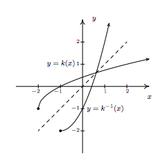
Graphically, everything checks out as well, provided that we remember the domain restriction on \(k^{-1}\) means we take the right half of the parabola.

Our last example of the section gives an application of inverse functions.

Example \(\PageIndex{4}\):demandfunctionofprice

Recall from Section 2.1 that the price-demand equation for the PortaBoy game system is \(p(x) = -1.5x + 250\) for \(0 \leq x \leq 166\), where \(x\) represents the number of systems sold weekly and \(p\) is the price per system in dollars.

1. Explain why \(p\) is one-to-one and find a formula for \(p^{-1}(x)\). State the restricted domain.
2. Find and interpret \(p^{-1}(220)\).
3. Recall from Section 2.3 that the weekly profit \(P\), in dollars, as a result of selling \(x\) systems is given by \(P(x)= -1.5x^2+170x-150\). Find and interpret \(\left( P \circ p^{-1}\right)(x)\).
4. Use your answer to part 3 to determine the price per PortaBoy which would yield the maximum profit. Compare with Example 2.3.3.

Solution

1. We leave to the reader to show the graph of \(p(x) = -1.5x + 250\), \(0 \leq x \leq 166\), is a line segment from \((0,250)\) to \((166,1)\), and as such passes the Horizontal Line Test. Hence, \(p\) is one-to-one. We find the expression for \(p^{-1}(x)\) as usual and get \(p^{-1}(x) = \frac{500-2x}{3}\). The domain of \(p^{-1}\) should match the range of \(p\), which is \([1,250]\), and as such, we restrict the domain of \(p^{-1}\) to \(1 \leq x \leq 250\).
2. We find \(p^{-1}(220) = \frac{500-2(220)}{3} = 20\). Since the function \(p\) took as inputs the weekly sales and furnished the price per system as the output, \(p^{-1}\) takes the price per system and returns the weekly sales as its output. Hence, \(p^{-1}(220) = 20\) means \(20\) systems will be sold in a week if the price is set at \( 220\) per system.
3. We compute \(\left( P \circ p^{-1}\right)(x) = P \left(p^{-1}(x)\right) = P\left(\frac{500-2x}{3}\right) = -1.5\left(\frac{500-2x}{3}\right)^2+170\left(\frac{500-2x}{3}\right)-150\). After a hefty amount of Elementary Algebra,\footnote{It is good review to actually do this!} we obtain \(\left( P \circ p^{-1}\right)(x) = -\frac{2}{3} x^2 +220x - \frac{40450}{3}\). To understand what this means, recall that the original profit function \(P\) gave us the weekly profit as a function of the weekly sales. The function \(p^{-1}\) gives us the weekly sales as a function of the price. Hence, \(P \circ p^{-1}\) takes as its input a price. The function \(p^{-1}\) returns the weekly sales, which in turn is fed into \(P\) to return the weekly profit. Hence, \(\left(P \circ p^{-1}\right)(x)\) gives us the weekly profit (in dollars) as a function of the price per system, \(x\), using the weekly sales \(p^{-1}(x)\) as the `middle man'.
4. We know from Section 2.3 that the graph of \(y = \left( P \circ p^{-1}\right)(x)\) is a parabola opening downwards. The maximum profit is realized at the vertex. Since we are concerned only with the price per system, we need only find the \(x\)-coordinate of the vertex. Identifying \(a = -\frac{2}{3}\) and \(b = 220\), we get, by the Vertex Formula, Equation 2.4, \(x = -\frac{b}{2a} = 165\). Hence, weekly profit is maximized if we set the price at \(\\)165\) per system. Comparing this with our answer from Example 2.3.3, there is a slight discrepancy to the tune of \(\\)0.50\). We leave it to the reader to balance the books appropriately. \(\( \Box \)\)