
10.2: Interactive Simulation with PyCX


( \newcommand{\kernel}{\mathrm{null}\,}\)
We can build an interactive, dynamic simulation model in Python relatively easily, using PyCX’s“pycxsimulator.py” file, which is available from http://sourceforge.net/projects/ pycx/files/ (it is also directly linked from the file name above if you are reading this electronically). This file implements a simple interactive graphical user interface (GUI) for your own dynamic simulation model, which is still structured in the three essential components—initialization, observation, and updating—just like we did in the earlier chapters.
To use pycxsimulator.py, you need to place that file in the directory where your simulation code is located. Your simulation code should be structured as follows:

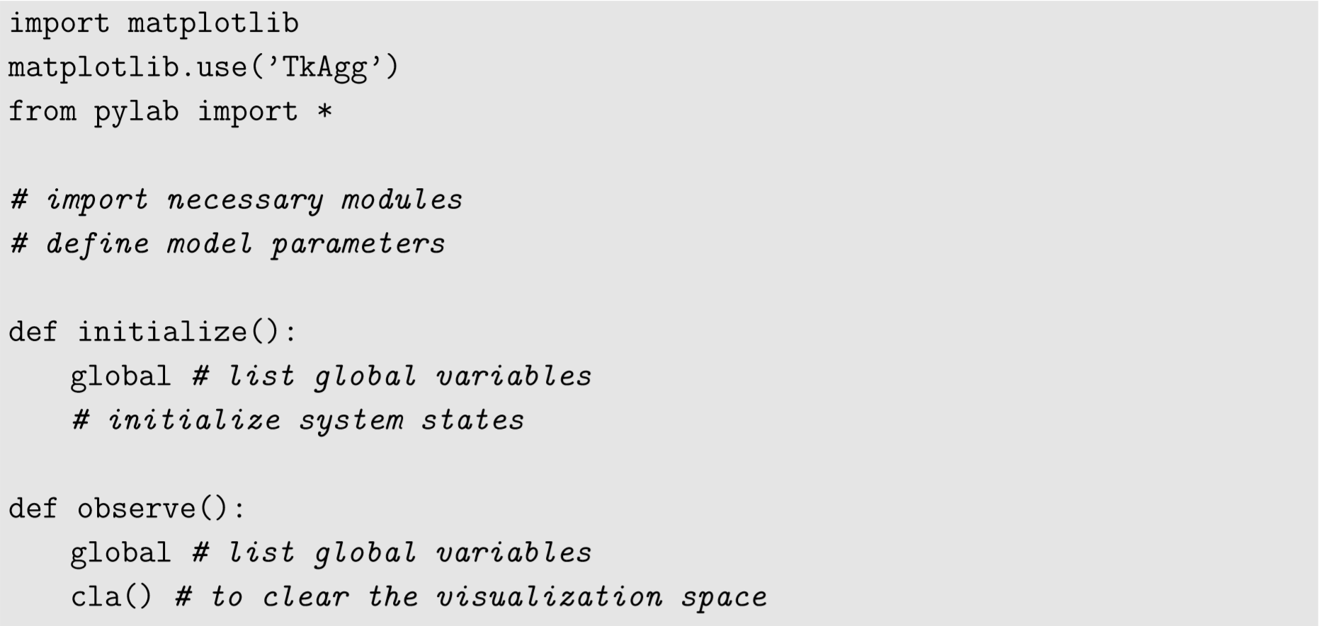
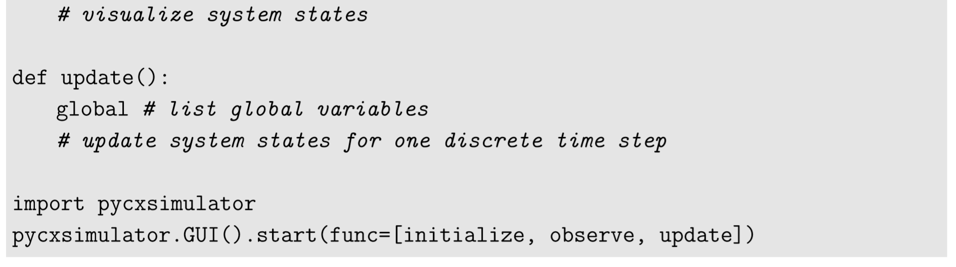
The first three lines and the last two lines should always be in place; no modification is needed.
Let’s work on some simple example to learn how to use pycxsimulator.py. Here we build a model of a bunch of particles that are moving around randomly in a twodimensional space. We will go through the process of implementing this simulation model step by step.
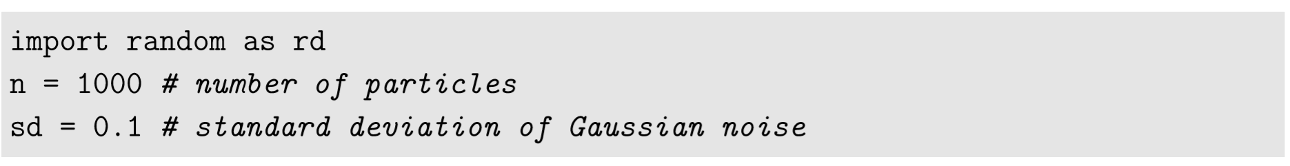
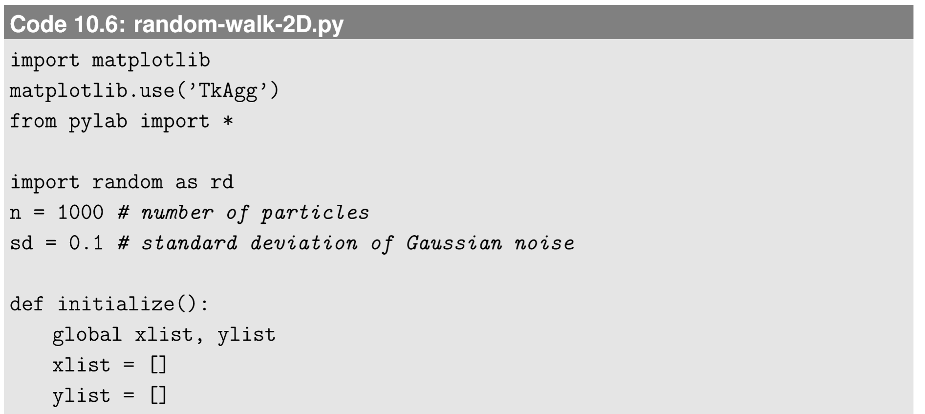
First, we need to import the necessary modules and define the parameters. In this particular example, a Gaussian random number generator is useful to simulate the random motion of the particles. It is available in the random module of Python. There are various parameters that are conceivable for this example. As an example, let’s consider the number of particles and the standard deviation of Gaussian noise used for random motion of particles, as model parameters. We write these in the beginning of the code as follows:

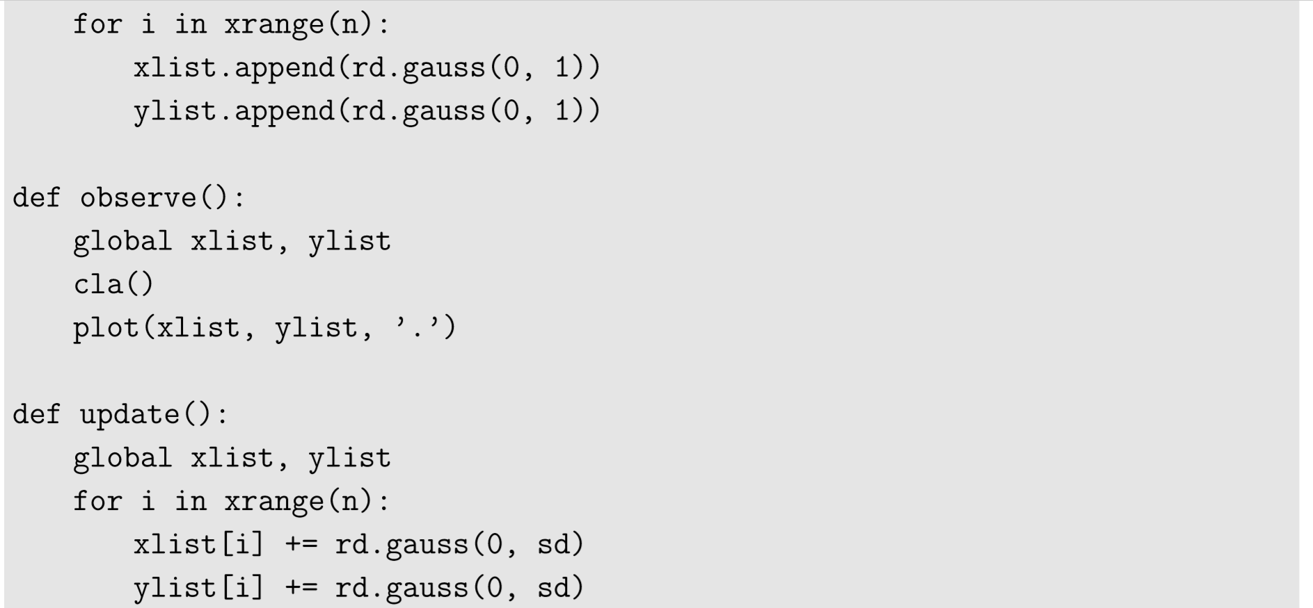
Next is the initialization function. In this model, the variables needed to describe the state of the system are the positions of particles. We can store their x− and y− coordinates in two separate lists, as follows:
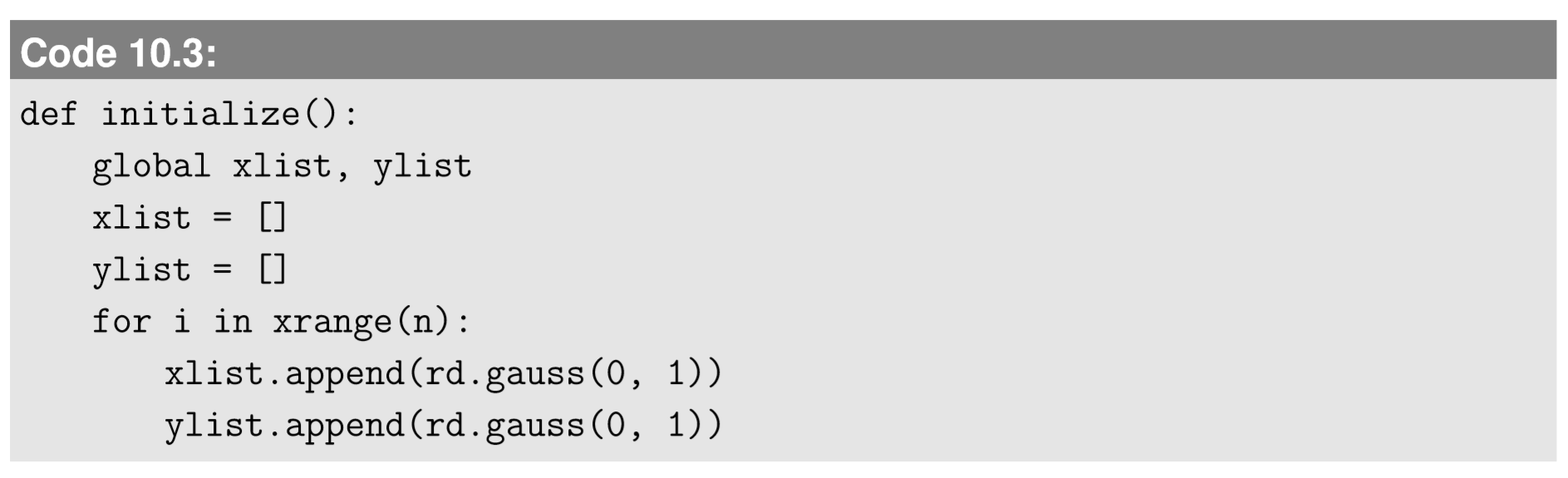
Here we generate n particles whose initial positions are sampled from a Gaussian distribution with mean 0 and standard deviation 1.
Then visualization. This is fairly easy. We can simply plot the positions of the particles as a scatter plot. Here is an example:
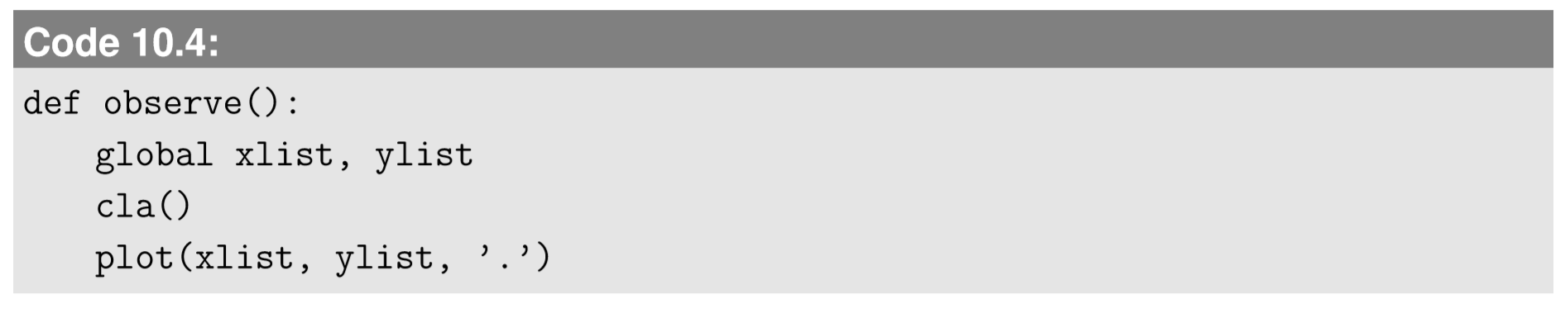
The last option, ’.’, in the plot function specifies that it draws a scatter plot instead of a curve. Finally, we need to implement the updating function that simulates the random motion of the particles. There is no interaction between the particles in this particular simulation model, so we can directly update xlist and ylist without using things like nextxlist or nextylist:
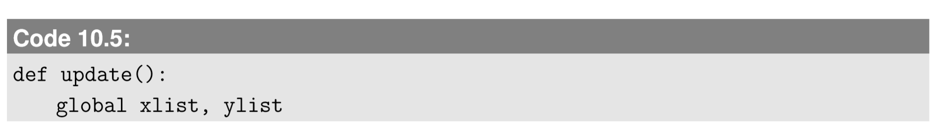
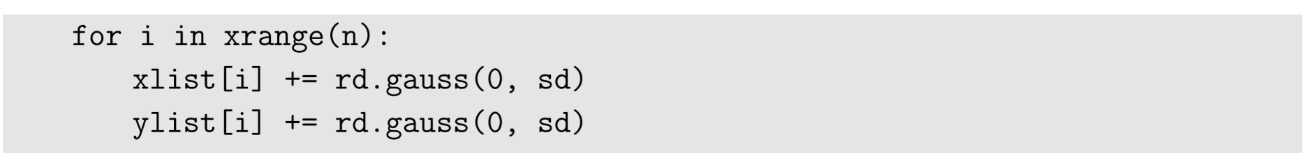
Here, a small Gaussian noise with mean 0 and standard deviation sd is added to the x− and y−coordinates of each particle in every time step. Combining these components, the completed code looks like this:

Run this code, and you will find two windows popping up (Fig. 10.1.1; they may appear overlapped or they may be hidden under other windows on your desktop)12.
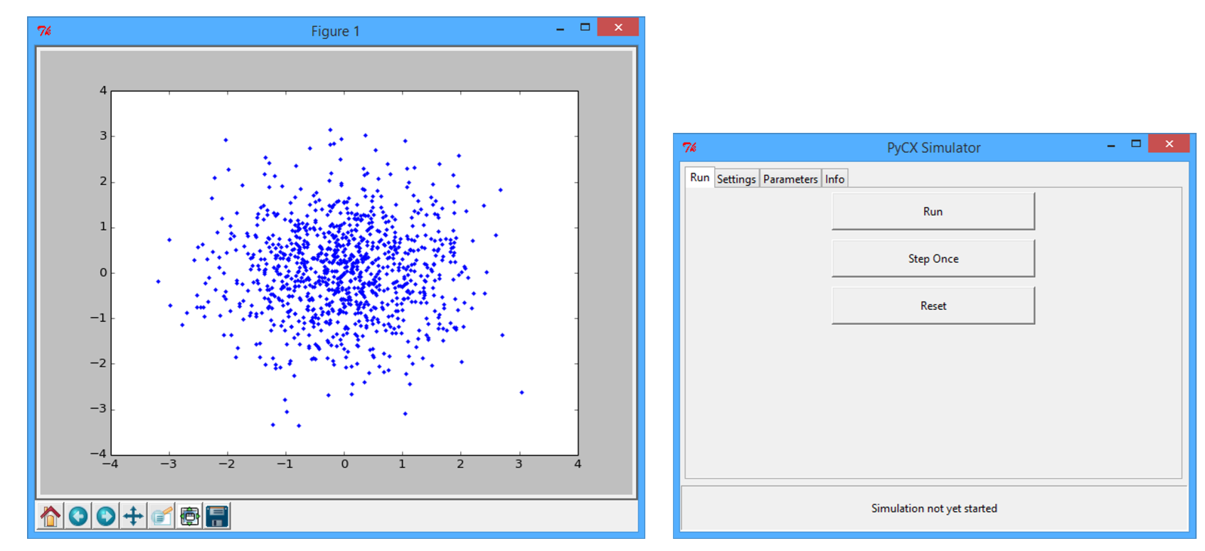
This interface is very minimalistic compared to other software tools, but you can still do basic interactive operations. Under the “Run” tab of the control window (which shows up by default), there are three self-explanatory buttons to run/pause the simulation, update the system just for one step, and reset the system’s state. When you run the simulation, the system’s state will be updated dynamically and continuously in the other visualization window. To close the simulator, close the control window.
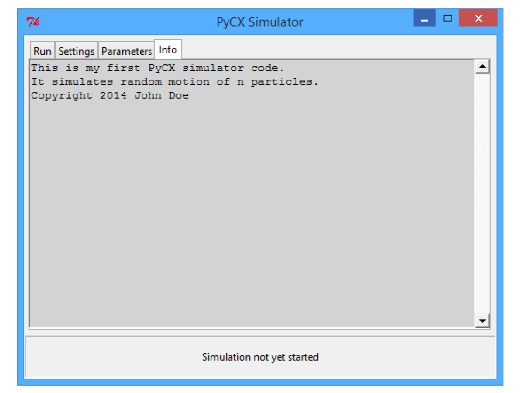
Under the “Settings” tab of the control window, you can change how many times the system is updated before each visualization (default = 1) and the length of waiting time between the visualizations (default = 0 ms). The other two tabs (“Parameters” and “Info”) are initially blank. You can include information to be displayed under the “Info” tab as a “docstring” (string placed as a first statement) in the initialize function. For example:
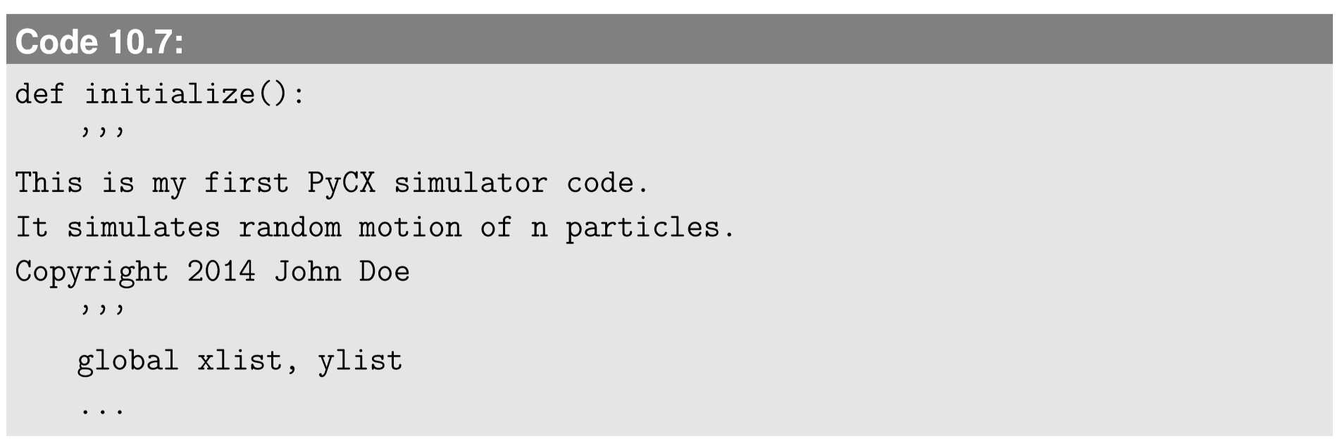
This additional docstring appears under the “Info” tab as shown in Fig. 10.1.2.
The animation generated by Code 10.6 frequently readjusts the plot range so that the result is rather hard to watch. Also, the aspect ratio of the plot is not 1, which makes it hard to see the actual shape of the particles’ distribution. Search matplotlib’s online documentation (http://matplotlib.org/) to find out how to fix these problems.
1If you are using Anaconda Spyder, make sure you run the code in a plain Python console (not an IPython console). You can open a plain Python console from the “Consoles” menu.
2If you are using Enthought Canopy and can’t run the simulation, try the following:
1. Go to “Edit”→“Preferences”→“Python” tab in Enthought Canopy.
2. Uncheck the “Use PyLab” check box, and click “OK.”
3. Choose “Run”→“Restart kernel.”
4. Run your code.
If it still doesn’t work, re-check the “Use PyLab” check box, and try again.