
12.2: Phase Space Visualization


- Last updated
- Apr 30, 2024
- Save as PDF

( \newcommand{\kernel}{\mathrm{null}\,}\)
If the phase space of a CA model is not too large, you can visualize it using the technique we discussed in Section 5.4. Such visualizations are helpful for understanding the overall dynamics of the system, especially by measuring the number of separate basins of attraction, their sizes, and the properties of the attractors. For example, if you see only one large basin of attraction, the system doesn’t depend on initial conditions and will always fall into the same attractor. Or if you see multiple basins of attraction of about comparable size, the system’s behavior is sensitive to the initial conditions. The attractors may be made of a single state or multiple states forming a cycle, which determines whether the system eventually becomes static or remains dynamic (cyclic) indefinitely.
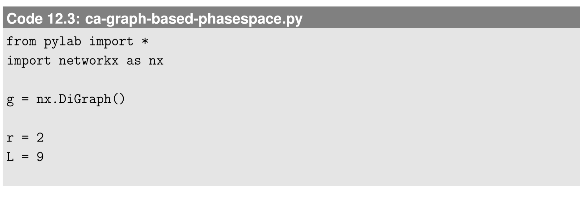
Let’s work on an example. Consider a one-dimensional binary CA model with neighborhood radius r = 2. We assume the space is made of nine cells with periodic boundary conditions(i.e., the space is a ring made of nine cells). In this setting, the size of its phase space is just 2^{9} = 512, so this is still easy to visualize.
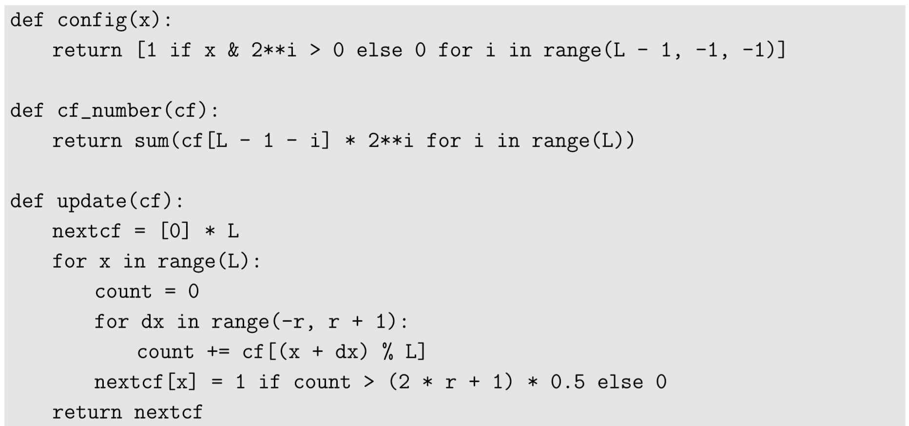
In order to enumerate all possible configurations, it is convenient to define functions that map a specific configuration of the CA to a unique configuration ID number, and vice versa. Here are examples of such functions:
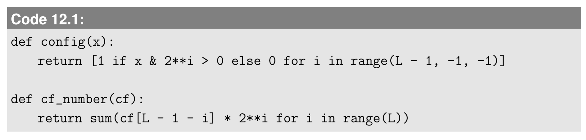
Here L and i are the size of the space and the spatial position of a cell, respectively. These functions use a typical binary notation of an integer as a way to create mapping between a configuration and its unique ID number (from 0 to 2^{L} −1; 511 in our example), arranging the bits in the order of their significance from left to right. For example, the configuration [0, 1, 0, 1, 1, 0, 1, 0, 1] is mapped to 2^{7} + 2^{5} + 2^{4} + 2^{2} + 2^{0} = 181. The function config receives a non-negative integer x and returns a list made of 0 and 1, i.e., a configuration of the CA that corresponds to the given number. Note that “&” is a logical AND operator, which is used to check if x’s i-th bit is 1 or not. The function cf_number receives a configuration of the CA, cf, and returns its unique ID number (i.e., cf_number is an inverse function of config).
Next, we need to define an updating function to construct a one-step trajectory of the CA model. This is similar to what we usually do in the implementation of CA models:
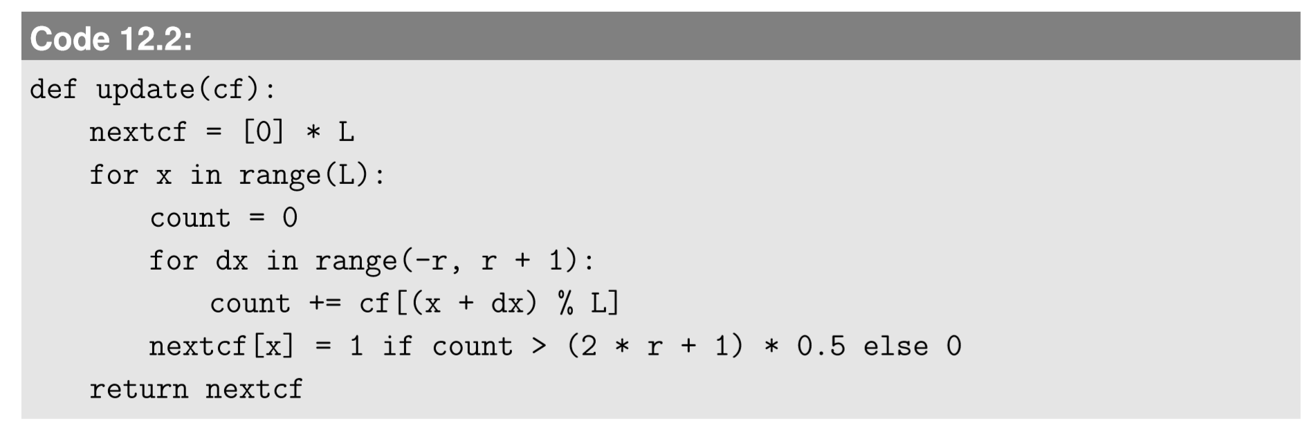
In this example, we adopt the majority rule as the CA’s state-transition function, which is written in the second-to-last line. Specifically, each cell turns to 1 if more than half of its local neighbors (there are 2r + 1 such neighbors including itself) had state 1’s, or it otherwise turns to 0. You can revise that line to implement different state-transition rules as well.
Now we have all the necessary pieces for phase space visualization. By plugging the above codes into Code 5.5 and making some edits, we get the following:
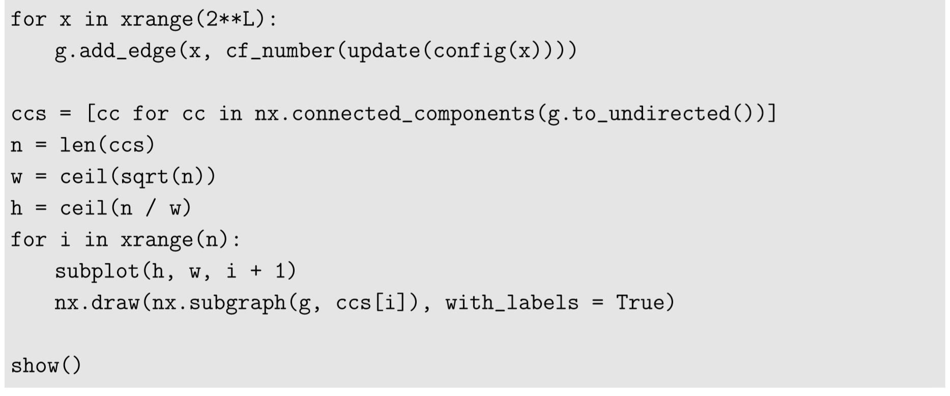
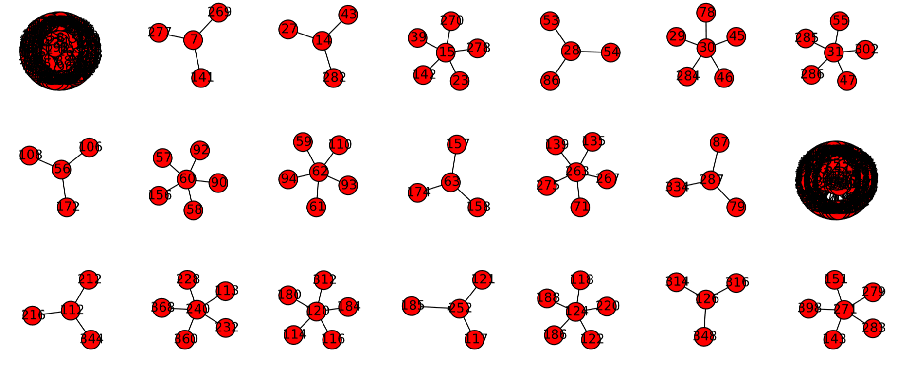
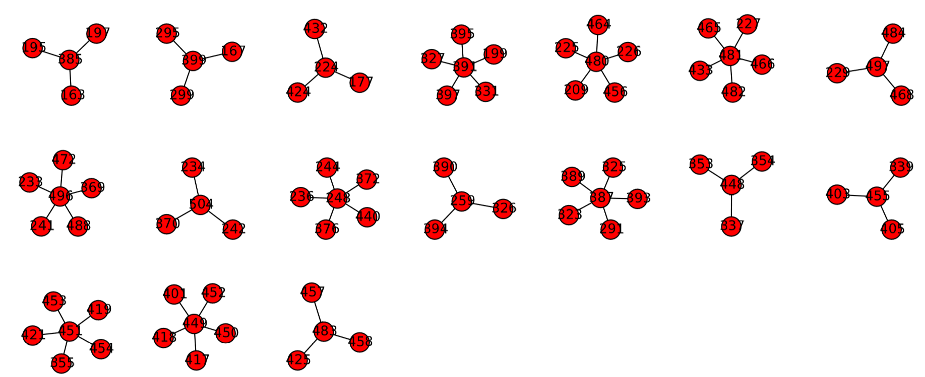
The result is shown in Fig. 12.2.1. From this visualization, we learn that there are two major basins of attraction with 36 other minor ones. The inside of those two major basins of attraction is packed and quite hard to see, but if you zoom into their central parts using pylab’s interactive zoom-in feature (available from the magnifying glass button on the plot window), you will find that their attractors are “0” (= [0, 0, 0, 0, 0, 0, 0, 0, 0], all zero) and “511” (= [1, 1, 1, 1, 1, 1, 1, 1, 1], all one). This means that this system has a tendency to converge to a consensus state, either 0 or 1, sensitively depending on the initial condition. Also, you can see that there are a number of states that don’t have any predecessors. Those states that can’t be reached from any other states are called “Garden of Eden” states in CA terminology.
Modify Code 12.3 to change the state-transition function to the “minority”rule, so that each cell changes its state to a local minority state. Visualize the phase space of this model and discuss the differences between this result and Fig. 12.2.1
The technique we discussed in this section is still na¨ıve and may not work for more complex CA models. If you want to do more advanced phase space visualizations of CA and other discrete dynamical systems, there is a free software tool named “Discrete Dynamics Lab” developed by Andrew Wuensche [47], which is available from http://www.ddlab.com/.