
14.1: Finding Equilibrium States


- Last updated
- Apr 30, 2024
- Save as PDF

( \newcommand{\kernel}{\mathrm{null}\,}\)
One nice thing about PDE-based continuous field models is that, unlike CA models, everything is still written in smooth differential equations so we may be able to conduct systematic mathematical analysis to investigate their dynamics (especially their stability or instability) using the same techniques as those we learned for non-spatial dynamical systems in Chapter 7.
The first step is, as always, to find the system’s equilibrium states. Note that this is no longer about equilibrium “points,” because the system’s state now has spatial extensions. In this case, the equilibrium state of an autonomous continuous field model
∂f∂t=F(f,∂f∂x,∂2f∂x2…)
is given as a static spatial function feq(x), which satisfies
0=F(feq,∂feq∂x,∂2f∂x2…).
A Simple Sinusoidal Source/Sink Model
For example, let’s obtain the equilibrium state of a diffusion equation in a 1-D space with a simple sinusoidal source/sink term:
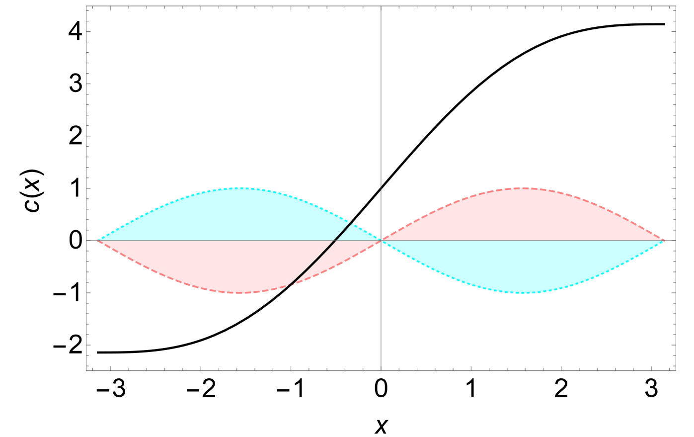
∂c∂t=D∇2c+sinx(−π≤x≤π)
The source/sink term sinx means that the “stuff” is being produced where 0<x≤π, while it is being drained where −π≤x<0. Mathematically speaking, this is still a nonautonomous system because the independent variable x appears explicitly on the right hand side. But this non-autonomy can be easily eliminated by replacing x with a new state variable y that satisfies
∂y∂t=0,
y(x,0)=x.
In the following, we will continue to use x instead of y, just to make the discussion easier and more intuitive.
To find an equilibrium state of this system, we need to solve the following:
0=D∇2ceq+sinx
=Dd2ceqdx2+sinx
This is a simple ordinary differential equation, because there are no time or additional spatial dimensions in it. You can easily solve it by hand to obtain the solution
ceq(x)=sinxD+C1x+C2
where C1 and C2 are the constants of integration. Any state that satisfies this formula remains unchanged over time. Figure 14.1.1 shows such an example with D=C1=C2=1.
Obtain the equilibrium states of the following continuous field model in a 1-D space:
∂c/∂t=D∇2c+1−x2
As we see above, equilibrium states of a continuous field model can be spatially heterogeneous. But it is often the case that researchers are more interested in homogeneous equilibrium states, i.e., spatially “flat” states that can remain stationary over time. This is because, by studying the stability of homogeneous equilibrium states, one may be able to understand whether a spatially distributed system can remain homogeneous or selforganize to form non-homogeneous patterns spontaneously.
Calculating homogeneous equilibrium states is much easier than calculating general equilibrium states. You just need to substitute the system state functions with constants, which will make all the derivatives (both temporal and spatial ones) become zero. For example, consider obtaining homogeneous equilibrium states of the following Turing pattern formation model:
∂u∂t=a(u−h)+b(v−k)+Du∇2u
∂v∂t=c(u−h)+d(v−k)+Dv∇2v
The only thing you need to do is to replace the spatio-temporal functions u(x,t) and v(x,t) with the constants ueq and veq, respectively:
∂ueq∂t=a(ueq−h)+b(veq−k)+Du∇2ueq
∂veq∂t=c(ueq−h)+d(veq−k)+Dv∇2veq
Note that,since ueq and veq no longer depend on either time or space, the temporal derivatives on the left hand side and the Laplacians on the right hand side both go away. Then we obtain the following:
0=a(ueq−h)+b(veq−k)
0=c(ueq−h)+d(veq−k)
By solving these equations, we get (ueq,veq)=(h,k), as we expected.
Note that we can now represent this equilibrium state as a “point” in a two-dimensional (u,v) vector space. This is another reason why homogeneous equilibrium states are worth considering; they provide a simpler, low-dimensional reference point to help us understand the dynamics of otherwise complex spatial phenomena. Therefore, we will also focus on the analysis of homogeneous equilibrium states for the remainder of this chapter.
Obtain homogeneous equilibrium states of the following “Oregonator” model:
ϵ∂u∂t=u(1−u)−u−qu+qfv+Du∇2u
∂v∂t=u−v+Dv∇2v
Obtain homogeneous equilibrium states of the following Keller-Segel model:
∂a∂t=μ∇2a−χ∇⋅(a∇c)
∂c∂t=D∇2c+fa−kc